Heave motion response of a floating offshore wind turbine with damping plate

저작자표시-비영리-변경금지 2.0 대한민국 이용자는 아래의 조건을 따르는 경우에 한하여 자유롭게 l 이 저작물을 복제, 배포, 전송, 전시, 공연 및 방송할 수 있습니다. 다음과 같은 조건을 따라야 합니다: l 귀하는, 이 저작물의 재이용이나 배포의 경우, 이 저작물에 적용된 이용허락조건 을 명확하게 나타내어야 합니다. l 저작권자로부터 별도의 허가를 받으면 이러한 조건들은 적용되지 않습니다. 저작권법에 따른 이용자의 권리는 위의 내용에 의하여 영향을 받지 않습니다. 이것은 이용허락규약(Legal Code)을 이해하기 쉽게 요약한 것입니다. Disclaimer 저작자표시. 귀하는 원저작자를 표시하여야 합니다. 비영리. 귀하는 이 저작물을 영리 목적으로 이용할 수 없습니다. 변경금지. 귀하는 이 저작물을 개작, 변형 또는 가공할 수 없습니다.

A thesisfor the degree ofDoctor of Philosophy

Heave motion response of a floating offshore

windturbine with damping plate

Hyeok-Jun Koh

Multidisciplinary Graduate School for Wind Energy

GRADUATE SCHOOL

JEJU NATIONAL UNIVERSITY

Heave motion response of a floating offshore wind

turbine with damping plate

Hyeok-Jun Koh

(Supervised by professor Il-Hyoung Cho)

A thesis submitted in partial fulfillment of the requirementfor the degree of

Doctor of Philosophy

2014. 6.

This thesis has been examined and approved by

---

Thesis director, Jong-ChulHur, Professor,Dept. of Mechanical Engineering

---

Yoon HyeokBae,AssistantProfessor,Dept. of Ocean System Engineering

---

Il-Hyoung Cho,Professor,Dept. of Ocean System Engineering

---

Dong-GukPaeng, Associate Professor,Dept. of Ocean System Engineering

---

Nam-Ho Kyong, Principal Researcher, Korea Institute of Energy Research

---

Date

Multidisciplinary Graduate School for Wind Energy

GRADUATE SCHOOL

iii

CONTENTS

CONTENTS ... iii

LIST OF FIGURES ...vi

LIST OF TABLES...xii

ABSTRACT ...xiii

Chapter 1 INTRODUCTION...1

1.1 Background and literature review ...1

1.2Objectives ...8

1.3Layout of thesis ...10

Chapter 2 ANALYTIC SOLUTION...12

2.1 A circular cylinder with a damping plate ...12

2.1.1 Diffraction problem...14

2.1.2 Radiation problem...20

2.2 A circular cylinder with a rigid and a porous damping plates ...23

2.2.1 Diffraction problem...25

2.2.2 Radiation problem...31

2.3 Equation of heave motion ...33

2.3.1 Frequency domain analysis ...33

2.3.2 Time domain analysis...34

iv

3.1 Free decay test...39

3.1.1 Introduction ...39

3.1.2Experimental set-up ...41

3.2 Model test in regular waves ...48

3.2.1 Introduction ...48

3.2.2Experimental set-up ...48

3.3 Model test in irregular waves ...51

3.3.1 Introduction ...51

3.3.2Experimental set-up ...51

Chapter 4 RESULTS AND DISCUSSION...58

4.1 Introduction...58

4.2 Comparisons ...59

4.3Free decay test...65

4.4Heave motion response in regular waves...68

4.5 Heave motion response in irregular waves ...74

Chapter 5 APPLICATION TO A FLOATING OFFSHORE WIND TURBINE USING FAST CODE...79

5.1 Introduction...79

5.2 Model...81

v

5.2.2 Platform...82

5.2.3 Environmental conditions...86

5.3 Results ...89

Chapter 6 CONCLUSIONS AND FUTURE WORK ...100

REFERENCES ...103

vi

LIST OF FIGURES

Fig. 1.1. Types of floating support platform. (a) Semi-submersible, (b) Spar, (c) TLP ...3 Fig. 1.2. Conceptual sketch of a cylinder with a damping plate. (a) a single rigid damping

plate, (b) dual (rigid and porous) damping plates...7 Fig. 2.1. Definition sketch of a circular cylinder with a damping plate. ...14 Fig. 2.2. Definition sketch of the circular cylinder with dual (rigid and porous) damping

plates. ...24 Fig. 3.1. Time history of heave motion by a heave free decay test. ...40 Fig. 3.2. The position of the cylinder with dual rigid damping plates for the heave free decay

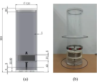
test in steel water. (a) equivalent position, (b) initial position with the 560g weight. ...41 Fig. 3.3. The experimental model. (a) 3D drawing, (b) fabricated shape...42 Fig. 3.4. Schematic sketch of the heave free decay test setup. (a) plane view, (b) elevation

view...44 Fig. 3.5. Wave generating system of the JNU wave tank. (a) piston-type wave maker, (b)

inclined porous plate wave absorber. ...44 Fig. 3.6. Vision tracking system. (a) targets of the model, (b) camera...45

vii

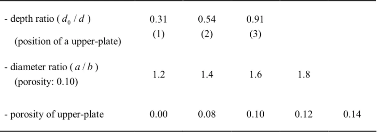
Fig. 3.7. Mooring configuration of the experimental model. (a) plane view, (b) elevation view. ...45 Fig. 3.8. The experimental model installed in the JNU wave tank. ...46 Fig. 3.9. Schematic drawings for the parameter selection of the damping plate attached on

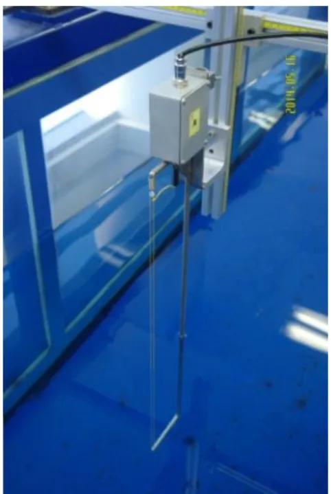
the experimental model. (a) position and diameter ratio, (b) porosity of the upper-plate...46 Fig. 3.10. Schematic sketch of the regular wave test setup. (a) plane view, (b) elevation view. ...49 Fig. 3.11. Capacitance-type wave gauge installed on the JNU wave tank. ...50 Fig. 3.12. The experimental model for the irregular wave test. (a) 3D drawing, (b) fabricated

model. ...52 Fig. 3.13. Schematic sketch of the irregular wave test setup...54 Fig. 3.14. Wave generating system of the SNU wave tank. (a) plunger-type wave maker, (b)

beach-type wave absorber. ...55 Fig. 3.15. Mooring configuration of the experimental model for the irregular wave test. ...55 Fig. 3.16. The experimental model installed in the SNU wave tank...56 Fig. 3.17. Measurement system. (a) accelerometer (AS-1GB), (b) surbo-type wave gauge. .56 Fig. 4.1. The S&N model. (a) definition sketch, (b) fabricated model. ...59 Fig. 4.2. Comparison of heave RAO of classic spar with a single damping plate from MEEM

viii

Fig. 4.3. Comparison of heave RAO of classic spar with dual rigid damping plates from MEEM with experimental and numerical results (Sudhakar and Nallayarasu, 2013)...61 Fig. 4.4. Heave added mass due to an oscillating classic spar with dual damping plates

according to the porosity of the upper-damping plate. ...63 Fig. 4.5. Heave damping coefficient due to an oscillating classic spar with dual damping

plates according to the porosity of the upper-damping plate...63 Fig. 4.6. Heave wave exciting force on the classic spar with dual damping plates according

to the porosity of the upper-damping plate. ...64 Fig. 4.7. Non-dimensional damping coefficients from the free decay test as function of

porosity and depth ratio for diameter ratio (a b/ = 1.6). ...66 Fig. 4.8. Non-dimensional damping coefficients from the free decay test as function of

diameter and depth ratio for porosity ( P = 0.1). ...67 Fig. 4.9. Comparison of heave RAO among analytic (MEEM), numerical (AQWA), and

experimental (Exp) results in case of cylinder only ( /a b =1.6). ...69

Fig. 4.10. Comparison of heave RAO among analytic (MEEM), numerical (AQWA), and experimental (Exp) results in case of cylinder with a single plate attached at the bottom of the circular cylinder ( /a b =1.6)...69

Fig. 4.11. Comparison of heave RAO between analytic (MEEM) and experimental (Exp) results in case of cylinder with dual rigid damping plates for different depth ratios

ix

of the upper-damping plate ( /a b =1.6)...70

Fig. 4.12. Comparison of heave RAO between analytic (MEEM) and experimental (Exp) results in case of cylinder with dual damping plates for different depth ratio of the porous ( P =0.1) upper-damping plate ( /a b =1.6). ...71

Fig. 4.13. Heave RAO of the circular cylinder with dual damping plates for different porosities of the upper-damping plate at position 1 ( /a b =1.6). ...72

Fig. 4.14. Heave RAO of the circular cylinder with dual damping plates for different porosities of the upper-damping plate at position 2 ( /a b =1.6). ...73

Fig. 4.15. Heave RAO of the circular cylinder with dual damping plates for different porosities of the upper-damping plate at position 3 ( /a b =1.6). ...73

Fig. 4.16. Heave motion time history of the circular cylinder without damping plate. (a) experiment, (b) MEEM. (case104: w_p=3.0 and H =0.102)...75_s

Fig. 4.17. Heave motion time history of the circular cylinder with damping plate. (a) experiment, (b) MEEM. (case203: w_p=3.0 and H =0.102, _s a b =1.6)...76/ Fig. 4.18. Comparison of wave and heave motion spectrum between analytic and

experimental results for the circular cylinder without the damping plate. ...77 Fig. 4.19. Comparison of wave and heave motion spectrum between analytic and

experimental results for the circular cylinder with a rigid damping plate...78 Fig. 5.1. Interfacing modules to achieve aero-hydro-servo-elastic simulation (Jonkman,

x

Fig. 5.2. Comparison of heave added mass due to an oscillating spar type floating platform

of the FOWT between analytical (MEEM) and numerical (AQWA) results. ...84

Fig. 5.3. Comparison of heave radiation damping due to an oscillating spar type floating platform of the FOWT between analytical (MEEM) and numerical (AQWA) results...84

Fig. 5.4. Comparison of heave wave exciting force on the spar type floating platform of the FOWT between analytical (MEEM) and numerical (AQWA) results. ...85

Fig. 5.5. Heave RAO for the spar type FOWT with a single and dual ( ) damping plates and without a damping plate. ...85

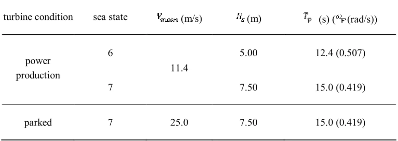
Fig. 5.6. JONSWAP wave spectrum ( ) for each sea state...87

Fig. 5.7. Wind speed time history ( , )...87

Fig. 5.8. Wave elevation time history ( , ). ...88

Fig. 5.9. Heave motion time history of the FOWT for sea state 6 (H =5.0 m, _s T =12.4 sec). p (a) without a damping plate, (b) with a single rigid damping plate (a b/ =1.6), (c) with dual (rigid + porous) damping plates (a b/ =1.6, d₀/d =0.54, P =0.1)...90

Fig. 5.10. Heave motion time history of the FOWT for sea state 7 (H =7.5 m, _s T =15.0 sec). p (a) without a damping plate, (b) with a single rigid damping plate (a b/ =1.6), (c) with dual (rigid + porous) damping plates (a b/ =1.6, d₀/d =0.54, P =0.1)...91

Fig. 5.11. Heave motion spectrum of the spar type FOWT with a single and dual (d₀/d =0.54, P =0.1) damping plates and without a damping plate (a b/ =1.6)

xi

for sea state 6 (H =5.0 m, _s T =12.4 sec). ...92p

Fig. 5.12. Heave motion spectrum of the spar type FOWT with a single and dual (d₀/d =0.54, P =0.1) damping plates (a b/ =1.6) and without a damping plate for sea state 7 (H =7.5 m, _s T =15.0 sec). ...93p

Fig. 5.13. The tower base axial force time history of the FOWT for sea state 7 (H =7.5 m, _s

p

T =15.0 sec). (a) without a damping plate, (b) with a single rigid damping plate

(a b/ =1.6), (c) with dual (rigid + porous) damping plates ( a b/ =1.6, 0 /

d d =0.54, P =0.1)...95

Fig. 5.14. The yaw bearing axial force time history of the FOWT for sea state 7 (H =7.5 m, _s

p

T =15.0 sec). (a) without a damping plate, (b) with a single rigid damping plate

(a b/ =1.6), (c) with dual (rigid + porous) damping plates ( a b/ =1.6, 0 /

d d =0.54, P =0.1)...96

Fig. 5.15. The blade root axial force time history of the FOWT for sea state 7 (H =7.5 m, _s

p

T =15.0 sec) in parked condition. (a) without a damping plate, (b) with a single

rigid damping plate (a b/ =1.6), (c) with dual (rigid + porous) damping plates (a b/ =1.6, d₀/d =0.54, P =0.1)...97

Fig. 5.16. The generated power time history of the FOWT for sea state 7 (H =7.5 m, _s

p

T =15.0 sec). (a) without a damping plate, (b) with a single rigid damping plate

(a b/ =1.6), (c) with dual (rigid + porous) damping plates ( a b/ =1.6, 0 /

xii

LIST OF TABLES

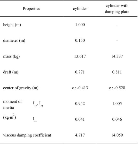
Table 3.1. The specification of the experimental model...42

Table 3.2. Experimental parameters in the free decay test. ...47

Table 3.3. The regular wave conditions ...50

Table 3.4. The specification of the experimental model for model test in irregular waves....53

Table 3.5. The irregular wave condition...57

Table 4.1. The specifications of the S&N model. ...60

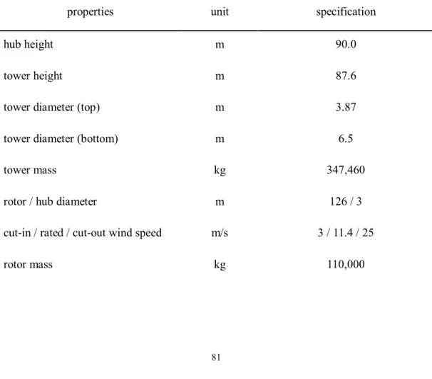
Table 5.1. Specifications of NREL 5MW wind turbine. ...81

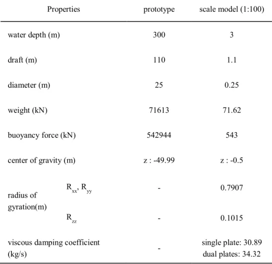
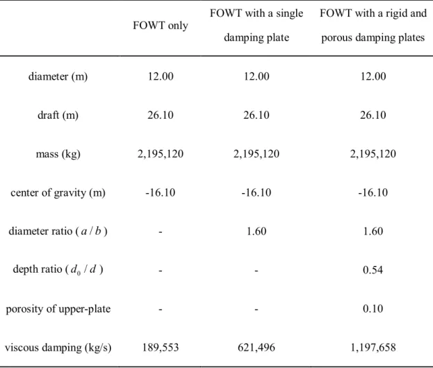
Table 5.2. Specifications of the spar type floating platform...83

Table 5.3. Environmental conditions for each sea state. ...86

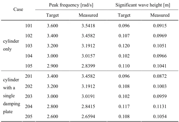
Table 5.4. Statistical analysis results of the wave and the heave motion of the FOWT. ...94

xiii

ABSTRACT

A rigid damping plate attached to the bottom of a cylinder has a distinct advantage in reducing the motion response of a floating circular cylinder by increasing the added mass and the damping coefficient. The added mass plays an important role in determining the location of the resonant frequency, and also the radiation damping reduces the motion amplitude at resonance. Furthermore, the porous holes of the permeable damping plate induce flow separation and vortices agitation,causingthe increase of the viscous damping and energy loss. To obtain better heave characteristics, the present research proposes dual damping plates: a porous upper-damping plate attached to the side wall of the cylinder and a rigid lower-damping plate to the bottom.

Analytical and experimental studies are carried out to investigate the heave motion response of the cylinder according to the characteristics of the damping plate such as depth ratio, diameter ratio, and porosity. The analytical method by using Matched Eigenfunction Expansion Method (MEEM) has been developed for the heave motion analysis of the floating circular cylinder with the single rigid or dual (a rigid anda porous)damping plates in the context of linear potential theory and Darcy’s law (the normal velocity of fluid passing through a thin porous disk is linearly proportional to the pressure difference across it).To apply the MEEM, the fluid domain is divided into three regions, and both the diffraction and the radiation potential in each region are expressed by the Fourier Bessel series. The unknown

xiv

coefficients in each region are determined by applying the continuity of the pressure and the normal velocity at the matching boundaries.With the assumption of an inviscid fluid in the potential theory, a heave viscous damping iscalculated by the non-dimensional damping coefficient obtained from aheave free decay test. In order to confirm the analytical solutions, experiments have been conducted in 2-D wave flume for the test in regular waves, and in large scaled wave flume for the test in irregular waves, with varying wave conditions.Theanalytical results are in good agreement with the experimental results in both regular and random waves, and the heave motion response of the cylinder is decreased drastically in the heave resonance region by the proposed dual damping plates.

In the application study of the damping plate to theFloating Offshore Wind Turbine (FOWT), the NREL offshore 5MW baseline wind turbine and spar type floating support structure are adopted to perform computational simulations using FAST code. The hydrodynamic input data of the floating support platform with a single rigid and dual(a rigid and a porous) damping platesfor HydroDyn,hydrodynamics module of FAST code, is calculated by the MEEM.The heave motion and the variation of the axial forces of the FOWT are considerably decreased ataround the heave resonantfrequency by the damping plate. It would be a great advantage to extend the fatigue life of the FOWT.In addition, it shifts the heave natural frequency to the lower frequency region due to the increase of the added mass. However, the decrease in the heave motion of the FOWT hardly affects the power generation.

1

Chapter 1

INTRODUCTION

1.1 Background and literature review

Major concerns of onshore wind turbine system such as noise, civil complaints, and spatial limitations bring the interest of offshore for an alternative installation site. Furthermore, an offshore environmental condition provides not only reducing the aerodynamic load by lower ground roughness, but also increasingthe capacity of wind turbine by avoiding such issues as transportation, installation, and visual effect.These are the reasons the offshore wind turbinehas come into the spotlight in the wind power industry. The offshore wind turbines installed to date are fixed type substructures by using monopile or conventional concrete gravity base in 20m depth of water, andtripod or jacket within40m depth of field.However, it affects fishing and sightseeing in coastal areas. Therefore, the development of deep water offshore wind farm bytheFloating Offshore Wind Turbine(FOWT) may be anticipated to be solved in order to overcome technical and economical weakness of the fixed type support structure.

The concept for large scale offshore floating wind turbines was introduced by Heronemus(1972).These systems could be deployed without any limitations of site conditions including high wind sites located further offshore in deep water. Numerous floating support platform configurations such as Spar, Tension Leg Platform (TLP), and

2

Semi-submersible used in the offshore oil and gas industries are possible for a FOWT (see Fig. 1.1).

For the design of theFOWT, the entire system composed of rotor, nacelle, tower, platform, and mooring system; subjected to wind, wave and hydrodynamic loads should be analyzed using integrated models (Nielson et al., 2006). Jonkman (2007) discussed dynamic response for theFOWT with a barge platform using an analytical model for Catenary mooring system.The specific properties of Hywind, the first full-scale spar type FOWT, provided by OC3 project have been used to analyze and investigate performance characteristics of the spar type FOWT by numerical (Nielsen et al., 2006; Skaare et al., 2007; Larsen and Hanson, 2007, Jonkman, 2009) and experimental (Shin, 2011; Myhr et al., 2011) methods.Waris and Ishihara (2012) developed a finite element model to investigate a dynamic response of floating offshore wind turbine system. Also, the effects of a single damping plate, applicability of linear and nonlinear models for dynamic response prediction of catenary and tension leg mooring system on floater response were discussed.

3

Fig.1.1. Types of floating support platform. (a) Semi-submersible, (b) Spar, (c) TLP

An analysis on hydrodynamic force by the movement of a floating structure has been carried out by many researchers. Havelock (1955) analyzed the added mass and damping coefficient of a sphere floating on the free surface using a multipole expansion method. Mei and Black (1969) solved the radiation problem and diffraction problem of a 2-D floating square structure. In order to reduce wave forces and motion of the floating structure, the majority of offshore platform structures have cylinder type substructures. Thus, the analysis of motion responses on a circular cylinder is one of the most important parts for the offshore

4

platform design. Bai (1977) presented numerical results for the added mass and damping of a semi–submerged two-dimensional heaving cylinder in the water of finite depth. The scattering problem of a cylinder was dealt with Garrett (1971) and the radiation problem was analyzed by Tung (1979) and McIver and Evans (1984). In addition, Kritis (1979) applied the hybrid method of Yeung (1975) to axisymmetric body and gave numerical results for a circular cylinder. Yeung (1981) gave the added mass and damping of a vertical cylinder in finite–depth waters.

An excessive heave motion is the result of a resonance which is generated when the natural frequency of the structure and the frequency of incident waves coincide. It is often to cause severe damage in mooring system. The basic concept of reducing the motion response of a floating structure is to increase the damping energy of the system by increasing the radiation and the viscous damping, or to move the natural frequency of the structure out of the frequency range of incident waves by increasing added mass.A damping plate installed at the bottom of the cylinder has a distinct advantage in reducing the motion responses of a floating circular cylinder by increasing the added mass and dampingas shown in Fig. 1.2 (a).Thiagarajan and Troesch (1998) observed the flow around the cylinder with a damping plate configuration using the particle image velocimetry(PIV) technique. Rho et al. (2002) carried out model tests to investigate the heave and pitch motion characteristics by the moon pool, strakes and a damping plate of a spar platform. Also they confirmed Mathieu-type instability which occurs when the pitch natural period is twice to the heave natural period.

5

Tao and Cai (2004) investigated vortex shedding pattern and hydrodynamic forces arising from the flow separation and vortex shedding around a damping plate of a circular cylinder by solving Navier-Stokes equation. Cho (2011) and Koh and Cho (2011) analyzed the hydrodynamic forces (added mass and the damping coefficient) acting on a cylinder with a damping plate using the Matched Eigenfunction Expansion Method (MEEM).

Tao et al. (2007) calculated viscous flow by a spar hull with two solid damping plates of variable spacings using a finite difference method. The results showed that a significant influence of the spacing of the plates on the hydrodynamic is revealed clearly when it is smaller than the critical value. At very small relative spacing, the configuration of the plates is found to produce lower damping and added mass than a cylinder with a single damping plate. It is caused that the vortex shedding process between the two plates is suppressed at very small relative spacing. Sudhakar and Nallayarasu (2013, 2014) investigated the influence of single and double damping plates on the hydrodynamic response of a spar in regular and irregular waves by the experimental study. A truss spar with several damping plates attached to a under the hull was proposed and investigated by numerical (Stansberg et al., 2001; Sadeghi et al., 2004) and experimental (Downie et al., 2000; .Magee et al., 2000) methods.

To obtain better heave motion characteristics, the dual–damping plate, which is composed of a porous plate attached to the side wall and a solid plate at the bottom of the cylinder is proposed (see Fig. 1.2). The porous damping plate can induce energy

6

dissipationby increasingviscous flow through holes. There have been many theoretical and experimental studies regarding the energy dissipation by porous plates. For example, the wave transmission of a thin vertical porous plate placed in deep water was investigated by Tuck(1975). He discussed the application of Darcy’s law for flows across porous plates and suggested that in the case of sinusoidal oscillations the velocity across the material with fine pores can be related to the pressure drop by a complex-valued frequency dependent parameter, which accounts for both viscous and inertial effects. The same porosity model was also used by Chwang(1983), Chwang and Wu(1994), Yu(1995), Wang and Ren(1994). Molin and Nielsen(2004) investigated the hydrodynamic characteristics of a perforated disk below the free surface based on the potential theory. They applied a quadratic relationship between the pressure difference and normal velocity. The amplitude dependent hydrodynamic coefficients are in good agreement with experimental results.In the case of wave interaction with submerged porous plates, the Darcy’s model was validated by Cho and Kim(2008) through small and large scale experiments.Tao and Dray(2008) investigated the hydrodynamic characteristics of oscillatory solid or porous disk using model–scale experiments.

7

Fig.1.2. Conceptual sketch of a cylinder with a damping plate. (a) asingle rigid damping plate, (b) dual (rigid andporous) damping plates.

8

1.2Objectives

The previous researches about single and dual rigid damping plates have been carried out using numerical and experimental methods. In the experimental study, however, it requires too much time and high cost. Numerical calculations also require enormous computational time. Thus, the heave motion response of the cylinder is examined through an analytical method applied by the MEEM with regard to the variation of the characteristics of the single rigid and dualdamping plates. In the MEEM calculation, fluid domain is divided into three regions, and the velocity potentials in each region are expressed by the Fourier–Bessel series. The unknown coefficients in each region are determined by applying the continuity of pressure and normal velocity at the matching boundaries.

So far, there are no previous studies about the porous damping plate, attached to a cylinder,asa motion reduction device.In this research, the heave motion characteristics of circular cylinder with the porous damping plate are investigated based on the potential theory.The energy dissipation effect due to the porous damping plate is modeled by Darcy’s law, which the normal velocity of fluid passing through a thin porous plate is linearly proportional to the pressure difference across it.The proportional coefficient, called porous parameter, was empirically determined from the experiments with the various types of porous plates by Cho and Kim (2008).

9

The viscous effect which is ignored by the assumption of the potential theory is considered experimentally for the analytical solution.The viscous damping is calculated from the non–dimensional damping coefficientobtained experimentally by a free decay test in still water. In addition, the verification is done for all analytical solution through model test in regular and irregular waves.

Finally, the NREL offshore 5MW baseline wind turbine model (Jonkman et al., 2009) and thespar type floating support platform, scaled up to 100 times the experimental model,with single and dual damping plates are considered as the application model.In order to predict the heave motion response of the FOWT, it is simulated by the FASTwind turbine dynamic simulation tool(Jonkman and Buhl, 2005) withhydrodynamic coefficient including added mass and radiation dampingwhich were generated by the MEEM.To take into account the viscosity of the damping plate, the viscous damping obtained by the free decay test in this research is added toHydroDyn, hydrodynamics module of FAST code.

10

1.3Layout of thesis

In the chapter, an introduction of the motivation and aims of this study are included. The literature reviews of research on the cylinder type floating body and motion reduction devices are also given.

Chapter 2 providesthe analytical formulationof matched eigenfunction expansion method for two cases, a cylinder with single damping plate and dual (rigid and porous) damping plates.

Chapter 3 describes the properties of the experimental models for the motion response tests in regular and irregular waves. Experimental setups of the heave free decay test and modeltest in regular and irregular waves are also given in this chapter.

In Chapter 4,the results of the heave motion of the circular cylinder with various damping platesfrom the series of experiments and analytical calculations are presented and discussed. In addition, the viscous damping coefficients measured fromthe heave free decay test is investigated by the comparisonswith thedepth ratio, the diameter ratio, and the porosity of the damping plate.

Chapter 5, the analytical results of the floating support structure with the damping plates are applied for the motion analysis of 5MW floating offshore wind turbine using FAST code.

11

Finally, concluding remarks and future studies related to the present work are given in Chapter 6.

12

Chapter 2

ANALYTIC SOLUTION

2.1 A circular cylinder with a damping plate

Using the MEEM, we solved the diffraction and radiation problem for a numerical model in which a circular damping plate with the diameter a was attached to the bottom of a cylinder with the radius b. For the analysis, the polar coordinate system

(

r, ,q z

)

is chosen with the origin on the undisturbed free surface and the z-axis pointing vertically upwards. The water depth is denoted by h, the distance between the bottom of the cylinder and seabed by c h d= - , and the draft of a cylinder by d (see Fig. 2.1). The monochromatic incident waves with an amplitude Aand the frequency wapproaches to the cylinder. The water is assumed to be incompressible and inviscid, so that the fluid particle motion can be described by the velocity potential. Assuming the harmonic motion of the frequency w , the velocity potential heave motion responsecan be written as_F( , , , ) Re_{r q z t =}

{

_f( , , )_{r q z e}-i tw

}

_{, Re}

{

i t

}

a

z= z e-w . In the present research, only a heave motion is considered. Therefore, the total velocity potential can be expressed by the sum of the diffraction and radiation potentials as follows:

( , , )r z D( , , )r z i za R( , ),r z

f q =f q - w f _(2.1)

13

D

f includes the incident wave potential f_I and the scatteringpotential f_S, i.e. f_D = + . f f_{I S}

The radiation potential is represented by f_R. Since the body is axisymmetric, the radiation problem is a function of randz.

The potential f_{D R,} satisfies Laplace’s equation (2.2) in the fluid and the following boundary conditions Eqs. (2.3–2.7).

2 , 0, in thefluid domain D R f Ñ = (2.2)

(

)

, 2 , 0, / on 0 D R D R K K g z z ¶f f w ¶ - = = = (2.3) , _{0, on} D R _{z h} z ¶f ¶ = = - (2.4) , 1/2 1 , lim D R 0, D R r r r ik f f ®¥ ¶ æ ö - = ç _¶ ÷ è ø (2.5) , _{0, on , 0} D R _{r b d z} r ¶f ¶ = = - £ £ (2.6) 0, on 0, 1, D R z _{r z d} z ¶f ¶ ¶f ¶ ì ₌ ïï _{< =} -í ï ₌ ïî (2.7)

14

Fig.2.1.Definition sketch of a circular cylinder with a damping plate.

2.1.1 Diffraction problem

To apply the MEEM, the fluid domain is divided into three regions, as shown in Fig. 2.1, i.e. (I) the outer region

(

r a³ - £ £ ; (II) the upper inner region of the damping , h z 0

)

plate

(

b r a£ £ - £ £, d z 0

)

; (III) the lower inner region of the damping plate

(

0£ £r a,- £ £ -h z d

)

. The diffraction potential is expressed by the separation of variables.

15 0 ( , , ) l ( , )cos . D D l igA r z r z l f q j q w ¥ = = -

å

(2.8)

In the outer region, the velocity potential satisfying Eqs.(2.2–2.5)can be written as:

( )

_{( )}

_{( )}

_{( )}

(

)

(

) ( )

1 1 1 0 10 1 0 1 , , l D l n D l l ln n n l n K k r r z J k r f z A f z K k a j b ¥ = = G +

å

(2.9)

whereG =0 N10/ coshk h1 and blis defined by 0 1, 2

( )

, 1

l

l i l

b

=

b

= ³ .

J

_lis the Bessel functions of the first kind andK is the modified Bessel functions of the second kind. The _l

eigenvalues k are the solution of the following dispersion equation. _1n

2 1ntan 1n , 0,1,2, k k h n g w = - = L (2.10)

where n=0,

(

k₁₀= -ik₁

)

term corresponds to an outgoing waves and n³1represents the evanescent waves. The eigenfunctions f_1n

( )

z in Eq. (2.9) are given by

( )

1

(

)

2 1 1 1 1 1 1 sin 2 1 cos , with 1 2 2 n n n n n n k h f z N k z h N k h - æ ö = + = _ç + _÷ è ø (2.11)

and also satisfy the following orthogonality.

( ) ( )

0 1 1 1 , n m mn h f z f z dz h

ò

- =d (2.12)

whered_mnis the Kronecker delta defined by dmn = if 1 m n= , and dmn= if 0 m n¹ .

16 be written as follows: ( )

_{( )}

₍

₎

(

)

(

)

(

)

( )

2 2 2 2 2 0 ₂ , , l D l n D ln l n l n n n _{l n} I k b r z B I k r K k r f z K k b j ¥ = æ ¢ ö ç ÷ = -ç ¢ ÷ è ø

å

(2.13)

whereI is the modified Bessel function of the first kind. The prime appearing in the _l

superscript denotes the derivative with respect to the argument. The eigenvalues

(

k20= -ik k n2, 2n, =1, 2,L

)

in the region (II) are the roots of the dispersion

relation

(

2

)

2ntan 2n /

k k d= -w g , and the normalized vertical eigenfunctions f_2n

( )

z are

defined as follows:

( )

1

(

)

2 2 2 2 2 2 2 sin 2 1 cos . with 1 . 2 2 n n n n n n k d f z N k z d N k d - æ ö = + = _ç + _÷ è ø (2.14)

With the above definitions for f_1n

( )

z , it can be easily shown that the eigenfunctions

satisfy the orthogonal relation.

( ) ( )

0 2 2 1 . n m mn df z f z dz d

ò

- =d (2.15)

In the region (III), the diffraction potential takes the following form.

( )

_{( )}

( )

( )

(

)

3 0 , cos , l D l n D n ln n n l n I r r z C z h I a l j e l l ¥ = =

å

+ (2.16)

17

the eigenvalues in the region (III) is ln=np/ ,c n

(

=0,1, 2,L

)

. The unknown coefficients D

ln A , D ln B , D ln C

(

n=0,1,2,L

)

in (2.9), (2.13), and (2.16) are determined by invoking the matching conditions. The continuity of velocity potential l

D j at r a= requires

( )

( )

( )

( )

(

)

2 0 1 0 10 1 0 0 , 0 cos , D ln ln n n D l l ln n n D n ln n n B s f z d z J k a f z A f z C z h h z d b e l ¥ ¥ = ¥ = = ì _{- £ £} ïï G + _{= í} ï _{+ £ £} -ïî

å

å

å

(2.17) where

(

)

(

)

(

)

(

)

2 2 2 2 . l n ln l n l n l n I k b s I k a K k a K k b ¢ = -¢

Multiplying both sides of Eq. (2.17) by the set of the functions

(

)

cosl_m z h+ , m=0,1,2,Land integrate with respect to zover

[

- - , the following h, d

]

equation can be obtained.

( )

1 0 0 0 , 0,1,2, D D lm ln mn l l m n C ¥ A G bJ k a G m = =

å

+ G = L (2.18) where

( )

(

)

1 1 cos . d mn _h n m G f z z h dz c l -=

ò

+

18

integrating with respect to zover

[

-d, 0

]

.

( )

1 0 0 0 _{, 0,1,2,} D ln mn l l m D n lm lm A H J k a H B m s b ¥ = + G =

å

= L (2.19) where

( ) ( )

0 1 2 1 . mn _d n m H f z f z dz d -=

ò

The continuity of l D r j ¶ ¶ atr a= also requires

( )

( )

( )

( )

(

)

2 0 1 1 1 0 10 0 1 , 0 cos 2 , n D ln ln n n D l l ln ln n _{D n} ln ln n f z B p d z f z d k J k a f z A q h z h C w h z d c b l ¥ ¥ = ¥ = = ì - £ £ ï ï ¢ _{G + = í} + ï _{£ £} -ïî

å

å

å

(2.20) where

(

)

(

)

(

)

(

)

2 2 2 2 2 , l n ln n l n l n l n I k b p k d I k a K k a K k b é ¢ ù ¢ ¢ ê ú = -¢ ê ú ë û

(

)

(

)

1 1 1 , n l n ln l n k hK k a q K k a ¢ =

( )

( )

. n l n ln l n cI a w I a l l l ¢ =

By multiplying both sides of Eq. (2.20) by f_1m

( )

z , m=0,1, 2,L and then integrating with respect to zover

[

-h, 0

]

, we obtain

19

( )

1 1 0 0 0 1 2 . D D D lm lm l l m ln ln nm ln ln nm n n A q bk hJ k a d ¥ B p H ¥ C w G = = ¢ = - G +

å

+

å

(2.21)

Using Eqs.(2.18) and (2.19), we obtain a system of equations

0 , , 0,1, 2, D D lmk D lm lm lk k lm lm F X A A l m q q ¥ = +

å

= = L (2.22) where 0 1 2 , ln nk nm lmk ln nk nm n ln n p H H F w G G s ¥ ¥ = = = -

å

-

å

( )

( )

1 0 0

( )

1 1 0 0 1 0 0 0 1 2 . ln l l n nm D lm l l m ln l l n nm n ln n p J k a H H X k hJ k a w J k a G G s b b d ¥ ¥ b = = G ¢ = - G +

å

+

å

G

For the numerical solutions of Eq. (2.22), the series are truncated after the Nth term. Thus, we have (N+1) unknowns of A_lmD. The unknowns constants B_lmD, C_lmD for the regions (II) and (III) can be determined from Eqs. (2.18) and (2.19).

From the solutions of the velocity potential, thevertical wave exciting force

{

}

(

Re 3

)

i t D

F ₌ X e-w _{on the bodycan be obtained by integrating the pressure over the damping} plate and the bottom of the cylinder in the region (II) and (III).

(

)

(

)

0(3) 0(2) 3 2 ₀ , , . a a D _b D X = prgA_êé rj r d dr- - rj r d dr- ù_ú ë

ò

ò

û (2.23)

20

2.1.2Radiation problem

The radiation problem by the vertical oscillation of the cylinder can be solved in a similar way as the diffraction problem. The velocity potential in the region (I) can be expressed by ( )

_{( )}

(

)

(

) ( )

1 0 1 1 0 0 1 , R n . R n n n n K k r r z A f z K k a f ¥ = =

å

(2.24)

The velocity potential in the regions (II) and (III) can be written as the sum of a particular solution and a homogeneous solution.

( )

_{( )}

_{( )}

₍

₎

(

)

(

)

(

)

( )

2 (2) 0 2 0 2 0 2 2 0 _{0 2} , , R n , R p n n n n n _n I k b r z r z B I k r K k r f z K k b f y ¥ = æ ¢ ö ç ÷ = + -ç ¢ ÷ è ø

å

(2.25) ( )

_{( )}

_{( )}

( )

( )

(

)

3 (3) 0 0 0 , , R n cos . R p n n n n n I r r z r z C z h I a l f y e l l ¥ = = +

å

+ (2.26)

The particular solutions in the region (II) satisfying the inhomogeneous body boundary condition can be written as follows:

( )2

_{( )}

_, 1_.

p r z z _K

y = + (2.27)

21 ( )3

_{( )}

1

₍

₎

2 2 , . 2 2 p r r z z h c y = é_ê + - ù_ú ë û (2.28)

The unknown coefficients A_nR , B_nR , C_nR can be determined by invoking the continuity of potential and normal velocity at r a= .

0 0 0 0 , R R mk R m m k k m m F X A A q q ¥ = +

å

= (2.29) where 0 0 0 0 1 2 , R n n nm m m n n nm n n n p h H X u w g G s ¥ ¥ = = = -

å

-

å

( )

_{( ) ( )}

0 ₂ 2 1 , , m _d p m h a z f z dz d - y =

ò

( )3

_{( ) ( )}

3 1 , , d m _h p m g a z f z dz c y -=

_ò

( )

( ) ( )

( )

( ) ( )

2 3 0 1 1 , , . d p p m _d m _h m a z a z u f z dz f z dz r r y - y - -¶ ¶ = + ¶ ¶

ò

ò

The radiation force resulting from the forced oscillation of the body can be found by integrating the pressure multiplied by the unit normal vector over the surface of the body. For the time harmonic motion of the angular frequency w , the radiation force

{

}

(

Re i t

)

R R

22

(

)

(

)

(3) (2) 33 33 0 2 a , a , , R R _b R i f ipwr rf r d dr rf r d dr iw m n w æ ö é ù = _êë - - - _úû= _ç + _÷ è ø

ò

ò

(2.30)

23

2.2 A circular cylinder with a rigid and a porous damping plates

We consider the diffraction and radiation problem of a circular cylinder attached with a rigid and a porous damping plates in a water depth h.The radius of the cylinder is assumed to be band the draft to be d . The rigid damping plate with the radius ais attached at the bottom of the cylinder and the porous circular plate, the radius of which is same as the rigid one, is fixed horizontally at a depth of d₀

(

d0<d

)

. It is also assumed that the fluid is incompressible and inviscid, so that the fluid particle motion can be described by a velocity potential F. For the introduction of velocity potential, we may assume that the flow separation through the openings and irrotational wakes remain confined within a short distance of the porous plate. This means that the openings must be small and distributed uniformly. The circular cylinder for the present model is described at Fig. 2.2. Assuming the harmonic motion of the frequency w, the velocity potential can be written as Eq. (2.1).

The potential f satisfies Laplace’s equation (2.2) in fluid; the free surface condition _{D R,} (2.3), the bottom condition (2.4), radiation condition (2.5), and the body boundary conditions Eqs. (2.6–2.7).

24

Fig.2.2. Definition sketch of the circular cylinder with dual (rigid and porous) damping plates.

To impose the boundary condition at the porous circular plate, we applied Darcy’s law. As stated, the normal velocity is continuous through the porous boundary and proportional to the pressure difference between two sides of the boundary. Hence, the boundary condition on the horizontal porous plate may be written as

(

)

, , , , , , on 0, D R D R D R D R D R n i z d b r a z z f f s f f + -- + ± ¶ ¶ = = + - = - £ £ ¶ ¶ (2.31)

wheren_{D R,} denotes the normal velocity at the bottom of the cylinder (nD =0,nR= ). The 1 superscript ±means the upper side of the porous plate and the lower side, respectively.

25

According to Mei et al.(1974), the imaginary part of s is related to the inertia effect and it may be neglected when the plate is thin and the size of holes is small. The imaginary part of

s is proportional to flow accelerations, and thus has nothing to do with energy dissipation. The positive real value of s represents viscous effects and can directly be obtained from experiments. The positive real value of s is called the porous-effect parameter

(

=r w mb₀ /

)

with b and ₀ m being the porosity coefficient and dynamic viscosity. The limiting case b₀® corresponds to the impermeable plate and 0 b₀® ¥ means that the plate is infinitely porous so that there is no obstruction in the fluid domain. The new dimensionless porosity parameter b used in the present numerical examples is defined as _por

follows: 0 1 1 2 2 . por b b k k pr w ps m = = (2.32)

After studying a systematic experimental investigation with a thin perforated steel plate in a 2-D wave tank, Cho and Kim(2008) suggested the empirical formula of

57.63 0.9717

por

b = P- where P and bpor where the porosity and porosity parameter,

respectively.

2.2.1 Diffraction problem

26

2.2i.e. (I) the outer region

(

r a³ - £ £ ; (II) the upper inner region of the rigid , h z 0

)

damping plate

(

b r a£ £ - £ £ ; (III) the lower inner region of the rigid damping , d z 0

)

plate

(

0£ £r a,- £ £ - . h z d

)

In the outer region r a³ , the velocity potential satisfying Eqs. (2.2–2.5)can be written as: ( )

_{( )}

_{( )}

_{( )}

(

)

(

) ( )

1 1 1 0 10 1 0 1 , . l D l n D l l ln n n l n K k r r z J k r f z A f z K k a j b ¥ = = G +

å

(2.33)

The eigenvalue k in Eq. (2.33) is the solutions of the dispersion relation Eq. (2.10). The _1n

eigenfunctions f_1n

( )

z in Eq. (2.33) are given at Eq. (2.11) and also satisfy the orthogonality Eq.

(2.12).

In the region (II), the diffraction potential which satisfies body boundary conditions can be written as follows: ( )

_{( )}

₍

₎

(

)

(

)

(

)

( )

2 2 2 2 2 0 ₂ , , l D l n D ln l n l n n n _{l n} J k b r z B J k r H k r f z H k b j ¥ = æ ¢ ö ç ÷ = -ç ¢ ÷ è ø

å

(2.34)

whereH is the Hankel function of the first kind. _l

The eigenfunctions f_2n

( )

z and eigenvalues k in the region (II) are the actual _2n

27 2 2 _0, d f f dz -k = % % _(2.35) 0, on 0 df Kf z dz- = = % % _(2.36)

(

)

0 0 0 0 , z d z d z d z d df df i f f dz =- + = dz =- - = s =- - - =- + % % % % _(2.37) 0, on df z d dz = = -% (2.38)

for the upper complex plane of k and0< < ¥s . Then, the following complex dispersion relation should be satisfied:

(

0

)(

0 0

)

(

)

sinh d d Kcosh d sinh d i Kcosh d sinh d .

k k - k -k k = s k -k k (2.39)

Eq. (2.39) can be rewritten as D

(

w k,

)

= , which is an implicit relation between the 0 wave number k and the frequency w. Since k k= ₁+ik₂ is a complex variable, the complex function D

(

w k,

)

can be separated by the real

(

DRe

(

w k

,

)

)

and imaginary part

(

)

(

DIm

w k

,

)

. Both the real and imaginary parts are to be zero.

(

,

)

Re

(

, ,1 2

)

Im

(

, ,1 2

)

0, D w k =D w k k +iD w k k = (2.40)

(

)

Re , ,1 2 0, D w k k = (2.41)

(

)

Im , ,1 2 0. D w k k = (2.42)

With the initial guesses

(

( )0 ( )0

)

1 , 2

28

(

,

)

0

D w k = can be easily solved by using the Newton-Raphson iteration method.

The infinite number of discrete solutions satisfying Eq. (2.39) are eigenvalues k . The _2n

resulting eigenfunctions f_2n

( )

z are

( )

₍

2

(

0

)(

2 2

₎

₍

2

)

₎

0

2

2 0 2 2 0 2 0

sinh cosh sinh , 0

cosh sinh cosh .

n n n n n n n n n k d d k k z K k z d z f z K k d k k d k z d d z d ì - + - £ £ ï = í _{- + - £} £-ïî (2.43)

By straightforward integration using Eq. (2.43), it can be shown that the eigenfunctions satisfy orthogonal relation.

( ) ( )

0 2 2 2 1 . n m m mn d f z f z dz N d

ò

- = d (2.44)

In the region (III), the diffraction potential takes the following form

( )

_{( )}

(

)

(

) ( )

3 3 3 0 3 , . l D l n D n ln n n l n I k r r z C f z I k a j ¥ e = =

å

(2.45)

The vertical eigenfunctions and eigenvalues in Eq. (2.45) are given by

( )

(

)

3n cos 3n . 3n n f z k z h k c p = + = (2.46) The continuity of l D j on r a= requires

29

( )

( )

( )

( )

( )

2 0 1 0 10 1 0 3 0 , 0 , D ln ln n n D l l ln n n D n ln n n B s f z d z J k a f z A f z C f z h z d b e ¥ ¥ = ¥ = = ì _{- £ £} ïï G + _{= í} ï _{£ £} -ïî

å

å

å

(2.47) where

(

)

(

)

(

)

(

)

2 2 2 2 . l n ln l n l n l n J k b s J k a H k a H k b ¢ = -¢

If we multiply (2.47) by f_3m

( )

z , m=0,1, 2,Land integrate with respect to zfrom

h

- to -d, the following equation can be obtained.

( )

1 0 0 0 , 0,1,2, D lm ln mn l l m n C ¥ A G bJ k a G m = =

å

+ G = L (2.48) where

( ) ( )

( )

₍

1 1

₎

1 3 _{2 2} 1 1 3 1 sin 1 . m d _{n n} mn _h n m n n m k k c G f z f z dz c N c k k -= =

-ò

Multiplying (2.47) by f_2m

( )

z , m=0,1, 2,L and integrating with respect to zover the region of validity

[

-d,0

]

.

( )

1 0 0 0 2 . 0,1, 2, D ln mn l l m D n lm lm m A H J k a H B m s N b ¥ = + G =

å

= L (2.49) The continuity of l D r j ¶ ¶ on r a= also requires

30

( )

( )

( )

( )

( )

2 0 1 1 1 0 10 ln 0 3 0 , 0 . n D ln ln n n D l l ln n D n n ln ln n f z B p d z f z d k J k a f z A q h f z C w h z d c b e ¥ ¥ = ¥ = = ì - £ £ ï ï ¢ _{G + = í} ï _{£ £} -ïî

å

å

å

(2.50) where

(

)

(

1

)

1 1 , l n ln n l n K k a q k h K k a ¢ =

(

)

(

)

(

)

(

)

2 2 2 2 2 , l n ln n l n l n l n J k b p k d J k a H k a H k b é ¢ ù ¢ ¢ ê ú = -¢ ê ú ë û

(

)

(

3

)

3 3 . l n ln n l n I k a w k c I k a ¢ =

If we multiply both sides of Eq. (2.50) by f_1m

( )

z , m=0,1, 2,L and then integrate both sides from -hto 0and use the orthogonal property of the eigenfunction f_1m

( )

z , the

following equation can be obtained.

( )

1 1 0 ln 0 1 2 , D D D lm lm l l m ln nm ln ln nm n n A q bk hJ k a d ¥ B p H ¥ C w G = = ¢ = - +

å

+

å

(2.51)

If substituting Eqs. (2.48) and (2.49) into Eq. (2.51), we obtain a system of equation

0 , D D lmk D lm lm lk k lm lm F X A A q q ¥ = +

å

= (2.52) where

31 0 2 1 2 , ln nk nm lmk ln nk nm n ln n n p H H F w G G s N ¥ ¥ = = = -

å

-

å

( )

ln

( )

1 0 0

( )

1 1 0 0 1 0 0 0 2 1 2 . l l n nm D lm l l m ln l l n nm n ln n n p J k a H H X k hJ k a w J k a G G s N b b d ¥ ¥ b = = G ¢ = - G +

å

+

å

G

Eq. (2.52) is the algebraic linear equation for the unknown coefficient D lm

A . The infinite matrix may be truncated at a certain term to solve the matrix equation numerically. By solving the above matrix equations, the unknown constants D

lm

B , D lm

C can be determined from Eqs. (2.48) and (2.49).

The wave exciting forces can be obtained by integrating the pressure over the body surface.

(

)

(

)

(

(

)

(

)

)

0(3) 0( 2) 0(2) 0(2) 3 2 ₀ , , , 0 , 0 . a a a D _b D _b D D X = prgA_êé rj r d dr- - rj r d dr- + r j r d- - -j r d- + drù_ú ë

ò

ò

ò

û (2.53)

2.2.2 Radiation problem

In the regions (II) and (III), the radiation potential can be written as the sum of a particular solution and a homogeneous solution. Therefore, the radiation potential in each three region can be written as:

32 ( )

_{( )}

(

)

(

) ( )

1 0 1 1 0 0 1 , R n , R n n n n K k r r z A f z K k a f ¥ = =

å

(2.54) ( )

_{( )}

( )

_{( )}

₍

₎

(

)

(

)

(

)

( )

2 2 0 2 0 2 0 2 2 0 _{0 2} , , R n , R p n n n n n _n J k b r z r z B J k r H k r f z H k b f y ¥ = æ ¢ ö ç ÷ = + -ç ¢ ÷ è ø

å

(2.55) ( )

_{( )}

( )

_{( )}

(

)

(

) ( )

3 3 0 3 3 0 0 3 , , R n . R p n n n n n I k r r z r z C f z I k a f y ¥ e = = +

å

(2.56)

The particular solutions in the regions (II) and (III) satisfy the inhomogeneous body boundary condition by Eqs. (2.27) and (2.28).

The unknown coefficients R n

A , R

n

B , R

n

C can be determined by Eq. (2.29).The radiation force in the heave mode is given by

(

)

(

)

(

(

)

(

)

)

(3) (2) (2) (2) 0 0 0 33 33 2 , , , , . a a a R R _b R _b R R f i r r d dr r r d dr r r d r d dr i i pwr f f f f n w m w - + é ù = _ê - - - + - - - _ú ë û æ ö = _ç + _÷ è ø

ò

ò

ò

(2. 57)

33

2.3 Equation of heave motion

Using Newton’s second law, the equilibrium between the inertia of the structure and the external forces can be written as:

,

R h D

Mz F&&= +F +F (2.58) whereM

(

=rSd

)

denotes the mass of the cylinder, z&& the second time derivative of the heave motion of the cylinder.F_h

(

= -rgS z

)

representsthe hydrostatic restoring force.

The equation of motion (2.58) can be rewritten as:

(

)

33 33

(M +

m

)&&z+ Bvis+

n

z&+

r

gS z F= D, (2.59)

where 2

( )

S =pa is the water-plane area. B is viscous damping coefficient, which is _vis

calculated from B_vis=2k r_d gS/w_o , where k is the non-dimensional damping coefficient _d and w_o

(

» rgS/

(

M+m₃₃

)

)

is the undamped natural frequency. The k can be determined _d from the freedecay test in still water.

2.3.1 Frequency domain analysis

34

decompose each term of Eq. (2.59) in spatial and temporal dependencies. Therefore, the equation of heave motion in the frequency domain is written by:

{

2

}

33 33 3

(M ) i B( _vis ) gS z_a X .

w

m

w

n

r

- + - + + = (2.60)

2.3.2Time domain analysis

The equation of heave motion of the cylinder in the time domain is expressed by integro-differential equation as follows (Cummins, 1962):

33 ₀

(M+m ( ))¥ &&z B z+ _vis&+

ò

tK( ) (t z t& -t t r)d + gS z F t= _D( ),(2.61) where the upper dots denote time derivatives.The integral in Eq. (2.61) is a memory term expressing the radiation wave damping, where the heave impulse response function K( )

t

can be calculated by functions of buoy frequency response by the inverse Fourier transform,

(

33 33

)

0 33 0 2 ( ) ( ) ( ) sin( ) 2 ( )cos( ) . K d d t m w m w wt w p n w wt w p ¥ ¥ = - - ¥ =

ò

ò

(2.62)

For the calculation of integral in Eq. (2.62), the entire frequency range is divided into a finite number of sub-domains and the integral can be expressed in terms of sum of integrals over N_p+ sub-domains 1 ( ,w wn n+₁) and (wN+1, )¥ . Then, the integral over each

35

sub-domain can be readily obtained by numerical integrations.

1 ( ) ( ) ( ), p N n n K t K t K¥ t = =

å

D + (2.63) where 1 1 33 33 2 ( ) ( )cos( ) , 2 ( ) ( )cos( ) . n n N n K d K d w w w t n w wt w p t n w wt w p + + ¥ ¥ D = =

ò

ò

For the numerical calculation of DK_n( )t , the radiation damping n w₃₃( )is to be approximated by the linear function within sub-domains ( ,w w_{n n}+₁)

33( ) a0 a1 , n n1 n w » + w w £ £w w₊ (2.64) where 33 1 33 1 0 1 33 1 33 1 1 ( ) ( ) , ( ) ( ) . n n n n n n n n n n a a n w w n w w w w n w n w w w + + + + + -= -=

-The contribution to the impulse response function from sub-domains can be written as

(

)

1 0 1 0 0 1 1 2 ( ) n cos( ) , n n K w a a d a P a P w t w wt w p + D »

ò

+ = + (2.65) where

36 1 1 1 0 1 1 1 1 2 sin( ) sin( ) 2 2 cos( ) ,

sin( ) sin( ) cos( ) cos( )

2 2 cos( ) . n n n n n n n n n n n n P d P d w w w w w t w t wt w p p t w w t w w t w t w t w wt w p p t t + + + + + + -æ ö = _{= ç ÷} è ø - -æ ö = = _ç + _÷ è ø

ò

ò

The contribution ranging(wN+₁, )¥ can be also calculated by a semi-analytical method. Since n w₃₃( ) should be vanish as w ® ¥, it can be approximated with an exponentially decay function 1 ( ) 33( ) e b w wN , n w »a - - + (2.66) where 33 1 33 1 33 1 ( ) 1 ( ), , ( ) N N N d d n w a n w b n w w + + + -= =

where

b

should be greater than 0 in order for n w₃₃( ) to vanish as w ® ¥. aand

b

are determined so that n w₃₃( ) and its first derivative is continuous at w w= _N+1 . The contribution ranging(w_N+₁, )¥ is then

1 1 ( ) 1 1 2 2 cos( ) sin( ) 2 2 ( ) N cos( ) . N N N K e b w w d w b w t t w t a t a wt w p + + p b t ¥ _{- - + +} ¥ æ - ö » = _{ç ÷} + è ø

ò

(2.67)

The memory term expressing as a time convolution integral in Eq. (2.61) can be evaluated using the trapezoidal integration with an impulse response function.