A Tailless UAV Multidisciplinary Design Optimization Using Global Variable Fidelity Modeling

(1)

Received: July 18, 2017 Revised: December 14, 2017 Accepted: December 14, 2017

662

http://ijass.org pISSN: 2093-274x eISSN: 2093-2480

Paper

Int’l J. of Aeronautical & Space Sci. 18(4), 662–674 (2017) DOI: http://dx.doi.org/10.5139/IJASS.2017.18.4.662

A Tailless UAV Multidisciplinary Design Optimization Using Global

Variable Fidelity Modeling

Maxim Tyan*

Department of Aerospace Information Engineering, Konkuk University, Seoul 05029, Republic of Korea

Nhu Van Nguyen**

Viettel Aerospace Institute, Viettel Group, Hanoi 100000, Vietnam

Jae-Woo Lee***

Department of Aerospace Information Engineering, Konkuk University, Seoul 05029, Republic of Korea

Abstract

This paper describes the multidisciplinary design optimization (MDO) process of a tailless unmanned combat aerial vehicle (UCAV) using global variable fidelity aerodynamic analysis. The developed tailless UAV design framework combines multiple disciplines that are based on low-fidelity and empirical analysis methods. An automated high-fidelity aerodynamic analysis is efficiently integrated into the MDO framework. Global variable fidelity modeling algorithm manages the use of the high-fidelity analysis to enhance the overall accuracy of the MDO by providing the initial sampling of the design space with iterative refinement of the approximation model in the neighborhood of the optimum solution. A design formulation was established considering a specific aerodynamic, stability and control design features of a tailless aircraft configuration with a UCAV specific mission profile. Design optimization problems with low-fidelity and variable fidelity analyses were successfully solved. The objective function improvement is 14.5% and 15.9% with low and variable fidelity optimization respectively. Results also indicate that low-fidelity analysis overestimates the value of lift-to-drag ratio by 3-5%, while the variable fidelity results are equal to the high-fidelity analysis results by algorithm definition.

Key words: Multidisciplinary Design Optimization (MDO), Variable fidelity optimization, Tailless aircraft, Unmanned Oerial

Vehicle (UAV), Aircraft conceptual design

1. Introduction

From the time of the first fliers, aviation engineers have sought an aircraft that will generate the maximum lift with the minimum drag. The relentless search for such an aircraft led to the creation of the flying wing (FW) concept. A FW aircraft is an aircraft without empennage and a fuselage; the entire payload is located inside the wing. The internal volume of such an aircraft should be large enough to allocate both subsystems and payload. Scientists and engineers have always showed their interest in aircraft of this scheme; however, just

a few of these FW aircraft have changed their status from experimental to operational. Inspired by the naturally stable glide of the Zanonia [1] seed in the early 1900s, J. W. Dunne was one of the first engineers to propose [2] the ideas of achieving inherent stability of a flying wing with his Dunne D.8 biplane. The Horten brothers designed several of the most advanced aircraft of the 1940s [3], including H0-229, the first jet-powered flying wing. Jack Northrop designed XB-35 and YB-35 heavy bombers after World War II. Although these aircraft were not mass-produced, test prototypes allowed designers to obtain a better understanding about the flying

This is an Open Access article distributed under the terms of the Creative Com-mons Attribution Non-Commercial License (http://creativecomCom-mons.org/licenses/by- (http://creativecommons.org/licenses/by-nc/3.0/) which permits unrestricted non-commercial use, distribution, and reproduc-tion in any medium, provided the original work is properly cited.

* Research Professor

** Deputy Director

*** Professor, Corresponding author: [email protected]

(2)

663

Maxim Tyan A Tailless UAV Multidisciplinary Design Optimization Using Global Variable Fidelity Modeling

http://ijass.org wing aerodynamics, stability and control.

In 1947, J. Northrop described the design issues of the scheme in his most well-known lecture [4]. A flying wing aircraft has a number of advantages compared to conventional aircraft. J. Northrop declared [4] that approximately 50% reduction of the parasitic drag coefficient(CD0) can be

achieved for a FW aircraft compared to conventional aircraft. Therefore, for a FW aircraft to achieve the same cruising speed as that of a conventional aircraft requires from 11 to 25% less power, and with the same amount of fuel, a FW aircraft can fly from 13 to 33% farther than conventional aircraft. Bolsunovsky et al. [5] estimated an approximately 20% increase in the lift-to-drag ratio (L/D) for a large passenger FW aircraft compared to a conventional one. In addition, to achieve better performance, the flying wing aircraft has a lower radar observability, which makes it more attractive for military applications because it can be invisible to enemy’s radar stations. However, a number of issues prevent the mass production of FW aircraft. The absence of a vertical tail leads to directional stability issues. Natural directional stability is impossible for FW aircraft. A level of directional stability compatible to that of conventional aircraft is achievable only with implementation of additional control devices, such as split drag rudders. The absence of a horizontal tail makes longitudinal control less efficient, which does not allow the aircraft to overcome a large nose-down pitching moment generated by high-lift devices, such as slotted flaps and slats at takeoff and landing. This fact leads to a lower maximum lift coefficient (CLmax), thus causing a longer takeoff and landing distance. A recent trend in the development of unmanned aerial vehicles (UAVs) and advances in automatic control systems has renewed the interest of engineers in the flying wing concept.

Currently, the objective of an aircraft design is to determine an optimum design considering multiple analysis disciplines. The process of aircraft design is a complex process that is composed of many different disciplines. From the early 1960s, it was clear that optimization of a single discipline cannot guarantee the overall optimum design [6]. The concept of multidisciplinary design optimization (MDO) was introduced in the 1980s to manage interdisciplinary connections in design optimization. Since then, MDO has been widely used in different fields of engineering design. However, the aircraft design methodology generally implements the empirical and semi-empirical equations based on Raymer [7], Roskam [8], Torenbeek [9] [10], Vortex Lattice Method (VLM) [11], and other relatively simple methods. These methods provide good prediction accuracy at the conceptual design stage for conventional fixed wing aircraft analysis. However, unconventional aircraft analysis

such as flying wing UCAVs or the analysis at transonic airspeeds may cause problems for low-fidelity codes. The increasing computational power of modern computer systems made it possible to use extensive computer simulations without significant effort, but the use of high-fidelity analysis tools for design optimization is still very limited. Pure high-fidelity optimization may require extensive use of supercomputers [12] [13] unless automatic differentiation [14] methods are used. Automation of the high-fidelity analysis process is another popular topic. High-fidelity aerodynamic analysis, also called computational fluid dynamics (CFD), is a process that involves several complex procedures for pre-and post-processing. This paper describes full automation of the CFD analysis process for a flying wing UCAV and its integration into a variable fidelity design optimization framework. The process involves configuration generation in the CAD program, structured computational grid generation, solution of the Reynolds averaged Navier-Stokes (RANS) equations and post-processing of the results.

Variable fidelity modeling (VFM), also known as variable complexity modeling (VCM), is an approach that combines high- and low-fidelity analysis tools to increase the analysis prediction accuracy while restricting the use of high-fidelity analysis with relatively low number. Many different VFM algorithms exist. Haftka [15] and Giunta [16] used a simple approach of scaling the low-fidelity function using a constant scaling factor. Alexandrov et al. [17] [18] developed VCM with approximation model management that implements a trust region management algorithm to enhance the convergence speed and guarantee convergence to a high-fidelity solution. Gano [19] [20] and Nguyen [21] independently introduced VF optimization algorithms that use the global approximation model (Kriging and Neural networks) to approximate the scaling function. Global variable fidelity modeling (GVFM) [22] is another approach that expands previously developed algorithms and improves the convergence speed and accuracy by introducing global design space initialization prior to starting the optimization loop with iterative refinement of the radial basis functions of the network-based global scaling model.

In this paper, the GVFM algorithm is introduced into the MDO environment to perform conceptual design optimization of a flying wing UCAV. The paper describes details of developed MDO framework with the focus on variable fidelity aerodynamic analysis. The framework relies on several well-known empirical and low-fidelity analysis methods. CFD analysis is introduced to enhance the accuracy of a FW UCAV multidisciplinary analysis. An efficient way to integrate a CFD analysis into aircraft conceptual design framework is proposed. MDO formulation includes

(3)

DOI: http://dx.doi.org/10.5139/IJASS.2017.18.4.662

₆₆₄

Int’l J. of Aeronautical & Space Sci. 18(4), 662–674 (2017)

methods provided by both variable and low fidelity analysis. The results section presents comparison between baseline aircraft characteristics, and two optimized configurations. The first one is optimized using low-fidelity analysis and the second with the proposed variable fidelity aerodynamic analysis.

2. Integrated Analysis Framework for UAV

Design

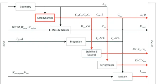
An integrated design synthesis program for a tailless aircraft conceptual design was developed in this study. This section describes details about the program. Fig. 1 shows the MDO framework flowchart. The overall program is composed of several interconnected disciplines. The analysis modules are developed based on empirical and semi-empirical equations, classical analysis methods that use simplified physical models with certain number of assumptions, and low-fidelity aerodynamic analysis.

2.1 Analysis Disciplines

This subsection describes details regarding each individual analysis module. Validation information for aerodynamic and mass analysis is presented. Aerodynamics and mass analysis are important because they supply the data for other analysis modules and affect the accuracy of the whole analysis. The user should provide geometric information sufficient to create the aircraft geometry through the input files. Several analysis modules require geometric data in their own format. For example, the mass analysis requires the sweep angle at the quarter chord line, while the aerodynamic analysis requires tip airfoil section offset in the longitudinal direction. The geometric analysis module

calculates the required parameters based on the user’s input and supports other analyses

A modified version of the Athena Vortex Lattice (AVL) code [23] by M. Drela and the in-house AERO09 [24] codes constitute the aerodynamic analysis module. AVL is a linear aerodynamic solver that uses the extended vortex lattice method to predict the aerodynamic characteristics of lifting surfaces. The framework also uses AVL to predict the stability and control (S&C) characteristics. AERO09 combines several existing methods adjusted for efficient prediction of the parasite drag of an aircraft at different speeds. The parasite drag of a FW is composed of friction, form, wave, and camber drag components. Parasite drag coefficient of a supersonic fighter aircraft with delta wing and single tail configuration measured in a wind tunnel is used to validate the AERO09 code. Fig. 2 shows a comparison of the parasite drag coefficients predicted by AERO09 and RDS [7] with the experimental data. The actual values of drag coefficient and details of configuration are not provided due to security issues. The present method exhibits good agreement with the reference wind tunnel data at subsonic and transonic speeds that are of interest in this study. Validation of the

low-Fig. 1: Integrated Analysis Program Flowchart

Fig. 1. Integrated Analysis Program Flowchart

34

Fig. 2: AERO09 Validation [23]

Fig. 2. AERO09 Validation [24]

(4)

665

http://ijass.org fidelity aerodynamic analysis is presented in section 2.2.

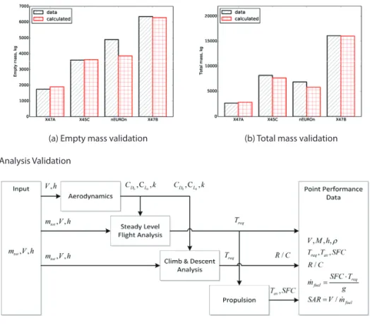
Statistical methods for fighter aircraft by D. Raymer [7] and for UAV by J. Gundlach [25] are the core analysis for tailless UAV mass and balance calculation. The mass of the wing fuselage and the subsystems are estimated using Raymer’s equations. A flying wing aircraft has no fuselage by definition; the root chord length and thickness are assumed as the length and diameter of a fuselage for mass estimation. Gundlach's equations are found to be more accurate for the landing gear mass calculation. The location of the aircraft center of gravity is calculated based on the location of each mass component. The CG of a wing and fuselage are assumed at 40% of mean aerodynamic chord and 45% of the fuselage length respectively as suggested by Raymer [7]. Location of a fuel tank CG and a payload is specified as the ratio of wingspan and ratio of a chord length. This approach allows changing the geometry of wing and preserving the safe location. CG of an engine is specified by user according to selected engine model. The user defines the mass and CG of an engine and payload explicitly. Fig. 3(a) and Fig. 3(b) show comparisons of the calculated and reference data for the takeoff gross mass and empty mass of a flying wing UCAV. The results show good agreement between the calculated data and the reference data, with a relative error of less than 5% for all aircraft models except for Dassault nEUROn.

Propulsion analysis calculates the turbofan engine’s fuel flow and the available thrust as a function of the engine sea

level thrust, altitude, Mach number and basic geometry parameters. The code implements the analysis methods of Mattingly [26]. This module is able to run direct analysis as well as table lookup of engine performance charts provided by the user.

The performance analysis module calculates the steady level flight and climb characteristics of an aircraft, such as the maximum speed, maximum rate of climb, speed for the maximum range and endurance. The point performance analysis process shown in Fig. 4 calculates thrust available, fuel flow, specific air range (SAR), rate of climb, and other parameters required to maintain steady level flight, climb or descending at a given altitude, speed, and with given aircraft mass.

Parameters such as the maximum speed, maximum specific range and minimum fuel flow are obtained by solving several optimization and root finding problems. For example, maximum speed is a speed when required thrust is equal to available thrust. The maximum and minimum speeds are calculated using Newton-Rhapson method by finding the root of the equation below.

8

as table lookup of engine performance charts provided by the user.

The performance analysis module calculates the steady level flight and climb characteristics of an aircraft, such as the maximum speed, maximum rate of climb, speed for the maximum range and endurance. The point performance analysis process shown in Fig. 4 calculates thrust available, fuel flow, specific air range (SAR), rate of climb, and other parameters required to maintain steady level flight, climb or descending at a given altitude, speed, and with given aircraft mass.

Fig. 4: Point Performance Analysis

Parameters such as the maximum speed, maximum specific range and minimum fuel flow are obtained by solving several optimization and root finding problems. For example, maximum speed is a speed when required thrust is equal to available thrust. The maximum and minimum speeds are calculated using Newton-Rhapson method by finding the root of the equation below.

( ) ( ) 0

req V T Vav

T   _. (1)

Required thrust is equal to aircraft drag in steady level flight. Drag at a given flight altitude, velocity and mass is provided by aerodynamic analysis. Propulsion analysis module calculates available thrust at a given altitude and Mach number. Equation is solved twice with initial velocity for the Newton-Rhapson method corresponding to Mach 0.1 to find the minimum and 0.9 to find the maximum speed.

Maximizing SAR at given aircraft mass and altitude provides a flight speed for the maximum range. The optimization formulation in this case as:

. (1)

Required thrust is equal to aircraft drag in steady level flight. Drag at a given flight altitude, velocity and mass is provided by aerodynamic analysis. Propulsion analysis module calculates available thrust at a given altitude and

Fig. 4: Point Performance Analysis

Fig. 4. Point Performance Analysis

35

a) Empty mass validation b) Total mass validation

Fig. 3: Mass and Balance Analysis Validation

(a) Empty mass validation (b) Total mass validation Fig. 3. Mass and Balance Analysis Validation

(5)

₆₆₆

Mach number. Equation is solved twice with initial velocity for the Newton-Rhapson method corresponding to Mach 0.1 to find the minimum and 0.9 to find the maximum speed.

Maximizing SAR at given aircraft mass and altitude provides a flight speed for the maximum range. The optimization formulation in this case as:

9 minimize subject to: : _fuel min max V m V  V V

Minimizing fuel flow in steady level flight provides a flight speed for the maximum endurance (loitering). The optimization formulation is:

minimize / subject to: : fuel min max V V m V  V V

The climb and descent point performance analysis calculates aircraft rate of climb and climb angle at a given speed, mass, altitude and thrust. The lift force for steady climb or descent flight is calculated as:

cos sin

L W



T



_. (2)

Rate of climb then

( / T )V R D W C   . (3)

Drag force at required lift, speed and altitude is calculated in aerodynamic analysis module. A flight path angle as:

1 /

sin R C V



_ 

. (4)

Actual values of ( / )R C and ( ) can be calculated by a fixed-point iteration. Initial assumption for the flight path angle is 0 degree. Fixed-point iteration converges within 3-5 iterations. Optimization formulation to find the maximum rate of climb at a given aircraft mass and altitude is:

maximize / subject to: : req a V v R C T T

Condition for the most economical climb is:

maximize ( )/ subject to : : fuel req av V R / C m T T

The mission analysis module is used to calculate the mission performance of an aircraft with a given configuration, mission profile and fuel mass. Different mission profiles may be composed of

minimize / subject to: : _fuel min max V V m V  V V

cos sin

L W



T



_. (2)

Rate of climb then

( / T )V R D W C   . (3)

1 /

sin R C V



_ 

. (4)

cos sin

L W



T



_. (2)

Rate of climb then

(

/ T )V

R C  _WD

. (3)

1 /

sin R C V



_ 

. (4)

(2) Rate of climb then

cos sin

L W



T



_. (2)

Rate of climb then

( / T )V R D W C   . (3)

1 /

sin R C V



_ 

. (4)

. (3)

9 minimize subject to: : fuel min max V m V  V V

cos sin

L W



T



_. (2)

Rate of climb then

(

/ T )V

R C  _WD

. (3)

1 /

sin R C V



_ 

. (4)

Actual values of (R/C) and (θ) can be calculated by a fixed-point iteration. Initial assumption for the flight path angle is 0 degree. Fixed-point iteration converges within 3-5 iterations. Optimization formulation to find the maximum rate of climb at a given aircraft mass and altitude is:

cos sin

L W



T



_. (2)

Rate of climb then

( / T )V R D W C   . (3)

1 /

sin R C V



_ 

. (4)

cos sin

L W



T



_. (2)

Rate of climb then

( / T )V R D W C   . (3)

1 /

sin R C V



_ 

. (4)

The mission analysis module is used to calculate the mission performance of an aircraft with a given configuration, mission profile and fuel mass. Different mission profiles may be composed of mission segments according to the user’s preference including cruise segments where range or endurance should be maximized within an available amount of fuel.

2.2 Variable Fidelity Aerodynamic Analysis

Aerodynamic analysis is extremely important for a flying wing aircraft multidisciplinary analysis. This discipline supplies data for almost all other analysis disciplines, as shown in Fig. 1, and it has a large effect on many characteristics of an aircraft. Equation (5) is used to estimate the total drag of an aircraft. Here, the drag polar is shown as a parabolic curve. The number of parameters that control the shape of the polar is three. These three parameters are

10

mission segments according to the user’s preference including cruise segments where range or endurance should be maximized within an available amount of fuel.

2.2 Variable Fidelity Aerodynamic Analysis

Aerodynamic analysis is extremely important for a flying wing aircraft multidisciplinary analysis. This discipline supplies data for almost all other analysis disciplines, as shown in Fig. 1, and it has a large effect on many characteristics of an aircraft. Equation (5) is used to estimate the total drag of an aircraft. Here, the drag polar is shown as a parabolic curve. The number of parameters that control the shape of the polar is three. These three parameters are (CD0, , and k CL0).

0 0 2 ( ) D CD k CL L C   C . (5)

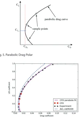
Three points can uniquely define a parabolic curve. The aerodynamic analysis results estimated at three different lift coefficients (angles of attack) can define the drag polar, as shown in Fig. 5. Thus, computationally expensive high-fidelity aerodynamic analysis results at three points can approximate the drag polar quite efficiently.

Fig. 5: Parabolic Drag Polar

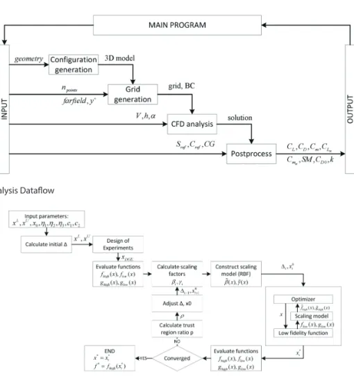
To validate the selected approach, low- and high-fidelity analyses with polar approximation were performed for a swept wing with an aspect ratio of 5.14, span of 0.9 meters, a quarter-chord sweep angle of 23 degrees, and 12-percent thick NACA64A312 airfoil. Fig. 6 shows a comparison of the experimental results [27] with the low-fidelity drag polar and the parabolic approximation constructed using high-fidelity data at three different angles of attack. The analysis is performed at sea level

10

mission segments according to the user’s preference including cruise segments where range or endurance should be maximized within an available amount of fuel.

2.2 Variable Fidelity Aerodynamic Analysis

Aerodynamic analysis is extremely important for a flying wing aircraft multidisciplinary analysis. This discipline supplies data for almost all other analysis disciplines, as shown in Fig. 1, and it has a large effect on many characteristics of an aircraft. Equation (5) is used to estimate the total drag of an aircraft. Here, the drag polar is shown as a parabolic curve. The number of parameters that control the shape of the polar is three. These three parameters are (CD0, , and k CL0).

0 0 2 ( ) D CD k CL L C   C . (5)

Fig. 5: Parabolic Drag Polar

To validate the selected approach, low- and high-fidelity analyses with polar approximation were performed for a swept wing with an aspect ratio of 5.14, span of 0.9 meters, a quarter-chord sweep angle of 23 degrees, and 12-percent thick NACA64A312 airfoil. Fig. 6 shows a comparison of the experimental results [27] with the low-fidelity drag polar and the parabolic approximation constructed using high-fidelity data at three different angles of attack. The analysis is performed at sea level

. (5)

To validate the selected approach, low- and high-fidelity analyses with polar approximation were performed for a swept wing with an aspect ratio of 5.14, span of 0.9 meters, a quarter-chord sweep angle of 23 degrees, and 12-percent thick NACA64A312 airfoil. Fig. 6 shows a comparison of the experimental results [27] with the low-fidelity drag polar and the parabolic approximation constructed using

high-Fig. 5: Parabolic Drag Polar

Fig. 5. Parabolic Drag Polar

Fig. 6: Aerodynamic Analysis Validation

Fig. 6. Aerodynamic Analysis Validation

(6)

667

http://ijass.org fidelity data at three different angles of attack. The analysis

is performed at sea level conditions and Mach number of 0.7 to match with experimental data. Low-fidelity analyses presented by a combination of AVL and AERO09 codes show good agreement with the experimental data at lift coefficients in the range of 0 to 0.1, whereas the prediction error at higher angles is observed to increase. Following the theory, it can be concluded that the (CD0) prediction by AERO09 is quite

accurate, while the induced drag predicted by AVL has lower accuracy. AVL models a wing as infinitely thin cambered plate. The compressibility effects that take place at high subsonic flight may not be calculated accurately. Parabolic approximation of a high-fidelity drag polar accurately follows the experimental data with mean absolute error of 1.9.10-3_.

Automation of a high-fidelity analysis process is a complex task since it involves several standalone programs that have different interfaces and automation schemes. An automated framework for CFD analysis is developed. The process includes generation of a CAD model using Dassault CATIA

_®

, structured computational grid generation using Pointwise

_®

, RANS CFD analysis using ANSYS Fluent

_®

, and post-processing. An interface that enables automated generation of a CAD model in CATIA is written in Python language

supported by CAA V5 CATIA API. The CAD generation module generates multi-segment tapered wing and exports the model for mesh generation. Parameters required to construct the model are airfoil coordinates for each section, length of the chords, incidence angles, leading edge sweep angles and spans of each segment. A set of automation scripts is written in Glyph language to enable mesh generation, setting a boundary conditions and solution export in the Pointwise software. Far-field distance in x, y, and z directions, number of nodes over the wing surface and at a far-field, and a minimum wall-distance (y+_{) are required to construct}

a C-type mesh in Pointwise. Another program interface is written in ANSYS text user interface (TUI) for automated import of a mesh, RANS CFD calculation, post processing and solution export. Atmospheric pressure, air density, flow speed at the far field and its direction are set through the TUI. After calculation is completed, ANSYS exports lift, drag, and moment coefficients to a text file. (CD0, k, and CL0) parameters

are then evaluated from 3-point parabola fit. (CLa, Cma) and a static margin evaluated by a central difference scheme. Fig. 7 shows the full process of high-fidelity aerodynamic analysis. 220×112×100 C-type computational mesh with (y+_{) of}

1.0 is used for CFD analysis. The CFD analysis of a single

39

Fig. 7: Automated CFD Analysis Dataflow

Fig. 7. Automated CFD Analysis Dataflow

Fig. 8: Global Variable Fidelity Modeling Process [21]

Fig. 8. Global Variable Fidelity Modeling Process [22]

(7)

₆₆₈

configuration at a single angle of attack takes approximately 6 hours on desktop PC with i7-4770 CPU and 32 GB RAM. Thus, polar approximation by 3 points takes about 18 hours. Analysis execution using ANSYS Fluent consumes the majority of computational resources. Automated process of CAD model generation, meshing and post processing takes less than a minute. On a contrast, the similar analysis with the proposed low-fidelity analysis setup consumes 3-5 seconds within the MDO framework written in Python language.

A variable fidelity modeling is an approach that allows for implementation of high-fidelity aerodynamic analysis into the design optimization to increase the prediction accuracy of a low-fidelity analysis code. In this research, variable fidelity aerodynamic analysis was implemented using Global Variable Fidelity Modeling (GVFM) [22] strategy. Fig. 8 shows the original process of GVFM.

An optimization process starts with the design of experiments (DOE) to construct a set of points that will form a scaling surrogate model. GVFM uses a radial basis functions (RBF) network with a Gaussian activation function to create a scaling model. Both high- and low-fidelity functions are evaluated at given DOE points. The surrogate model is then created using scaling factors (β) at each point.

13

An optimization process starts with the design of experiments (DOE) to construct a set of points that will form a scaling surrogate model. GVFM uses a radial basis functions (RBF) network with a Gaussian activation function to create a scaling model. Both high- and low-fidelity functions are evaluated at given DOE points. The surrogate model is then created using scaling factors ( ) at each point.

i i

i yHF yLF



 

. (6)

Here (yHF_i) and (yLFi) are the values of high and low-fidelity functions at point ( )x . The next i

stage is an optimization process that uses an approximation of a high-fidelity function instead of a low-fidelity function. An approximate high-fidelity function is called a scaled function. The following equation shows the calculation of a scaled function value.

( ) ( ) ( )

high low

f x  f x 



x

. (7)

Where f_high( )x is the scaled function, f x is a low fidelity function, and ( )low( )  x is a scaling

. (6)

Here (yHFi) and (yLFi) are the values of high and low-fidelity functions at point (xi). The next stage is an optimization

process that uses an approximation of a high-fidelity function instead of a low-fidelity function. An approximate high-fidelity function is called a scaled function. The following equation shows the calculation of a scaled function value.

13

An optimization process starts with the design of experiments (DOE) to construct a set of points that will form a scaling surrogate model. GVFM uses a radial basis functions (RBF) network with a Gaussian activation function to create a scaling model. Both high- and low-fidelity functions are evaluated at given DOE points. The surrogate model is then created using scaling factors ( ) at each point.

i i

i yHF yLF



  _. (6)

Here (yHF_i) and (yLFi) are the values of high and low-fidelity functions at point ( )x . The next i

stage is an optimization process that uses an approximation of a high-fidelity function instead of a low-fidelity function. An approximate high-fidelity function is called a scaled function. The following equation shows the calculation of a scaled function value.

( ) ( ) ( )

high low

f x  f x 



x _. (7)

Where f_high( )x is the scaled function, f x is a low fidelity function, and ( )_low( )  x is a scaling

, (7)

where f high(x) is the scaled function, f low(x) is a low fidelity

function, and β(x) is a scaling surrogate model. When the optimization is completed, a high-fidelity function is evaluated at an optimum point. If the predictive error

evaluated by equation (8) is large, then a new point is added to a scaling surrogate model and the optimization starts again.

14

surrogate model. When the optimization is completed, a high-fidelity function is evaluated at an optimum point. If the predictive error evaluated by equation (8) is large, then a new point is added to a scaling surrogate model and the optimization starts again.

| high( ) high( ) |

error f x f x _. (8)

The iteration continues until the difference between the prediction errors becomes less than the tolerance defined by the user. When convergence criterion is met, the algorithm terminates with the final solution ₍ *_, _{( )).}*

high

f x

x Therefore, the values of the objective and constraints are equal to the values of high-fidelity functions at the optimum point.

Fig. 9: Variable Fidelity Aerodynamic Analysis

Fig. 9 shows the variable fidelity aerodynamic analysis module that is implemented in the integrated analysis framework. Five scaling models compose the core of the variable fidelity analysis. The GVFM algorithm manages the initialization and update procedure of the scaling models. With the given aircraft geometry, aircraft velocity, angle of attack and flight altitude, the aerodynamic analysis calculates (CD0, , k CL0,L / D and, SM ).

3. UCAV Design

3.1 Optimization Formulation

Because a flying wing aircraft is an unconventional configuration, it is difficult to obtain information related to its stability and control and performance. As a result, several design objectives

. (8)

The iteration continues until the difference between the prediction errors becomes less than the tolerance defined by the user. When convergence criterion is met, the algorithm terminates with the final solution

14

surrogate model. When the optimization is completed, a high-fidelity function is evaluated at an optimum point. If the predictive error evaluated by equation (8) is large, then a new point is added to a scaling surrogate model and the optimization starts again.

| _high( ) _high( ) |

error f x f x _. (8)

The iteration continues until the difference between the prediction errors becomes less than the tolerance defined by the user. When convergence criterion is met, the algorithm terminates with the final solution ₍ *_, _{( )).}*

high

f x

x Therefore, the values of the objective and constraints are equal to the values of high-fidelity functions at the optimum point.

Fig. 9 shows the variable fidelity aerodynamic analysis module that is implemented in the integrated analysis framework. Five scaling models compose the core of the variable fidelity analysis. The GVFM algorithm manages the initialization and update procedure of the scaling models. With the given aircraft geometry, aircraft velocity, angle of attack and flight altitude, the aerodynamic analysis calculates (CD0, , k CL0,L / D and, SM ).

3. UCAV Design

3.1 Optimization Formulation

Because a flying wing aircraft is an unconventional configuration, it is difficult to obtain information related to its stability and control and performance. As a result, several design objectives

. Therefore, the values of the objective and constraints are equal to the values of high-fidelity functions at the optimum point.

Figure 9 shows the variable fidelity aerodynamic analysis module that is implemented in the integrated analysis framework. Five scaling models compose the core of the variable fidelity analysis. The GVFM algorithm manages the initialization and update procedure of the scaling models. With the given aircraft geometry, aircraft velocity, angle of attack and flight altitude, the aerodynamic analysis calculates (CD0, k, CL0, L/D, and SM).

3. UCAV Design

3.1 Optimization Formulation

Because a flying wing aircraft is an unconventional configuration, it is difficult to obtain information related to its stability and control and performance. As a result, several design objectives and constraints are selected based

Fig. 9. Variable Fidelity Aerodynamic Analysis

Fig. 10: Suppression of Enemy Air Defenses (SEAD) Mission Profile [31]

Fig. 10. Suppression of Enemy Air Defenses (SEAD) Mission Profile [32]

(8)

669

http://ijass.org on comparison with manned aircraft of a similar category

and dimensions. The objective of maximizing the lift-to-drag ratio (L/D) is common for aircraft design optimization problems. Longitudinal stability of an aircraft is constrained by the static margin. Nicolai [28] provided the values of the static margin for a Northrop T-38 trainer and a Douglas F4D carrier-based fighter as 5% and 3%, respectively. The design of a UCAV considered in this study has a positive static stability and a static margin constraint set between 5 and 15%, which is slightly higher than that of manned fighter aircraft. The low speed condition constrains the elevator authority and the wing area. The trim angle of attack is restricted by 8 degrees and the elevator deflection to trim to -20 to 20 degrees at a speed of 65 m/s at sea level. One of the main issues of a flying wing is a directional stability [4] [29] [30] [31]. Achieving a level of directional stability similar to that of conventional

aircraft is not possible without implementation of special control devices. It is decided to maintain positive inherent directional stability, for clean configuration at the level of (Cnβ≥0.003). The lateral stability criterion is set to the level of a Northrop T-38 aircraft: (Clβ≤-0.075). However, the solution is typically restricted by directional stability rather than lateral stability. The minimum combat radius for a suppression of enemy air defense (SEAD) [32] mission profile is constrained to 750 km. Fig. 10 and Table 1 present details about the selected mission profile. The cruise altitude is 10 km. The range is maximized at segments C and I. A summary of all of the design requirements is presented in Table 2 regarding the design formulation.

Two design problems are solved in this study. The first one implements pure low-fidelity optimization and the second one use the GVFM aerodynamic model in an MDO loop. Table 1. Mission Profile Segments Table 1: Mission Profile Segments

Segment Segment

A Takeoff at sea level G Withdrawal at 540 kts (277.8 m/s)

B Climb from sea level to cruise altitude H Climb from withdrawal to cruise altitude

C Cruise (maximum range) I Cruise (maximum range)

D Descent to 20,000 ft (6096 m) J Descent from cruise altitude to sea level E Penetration at 540 kts (277.8 m/s) K Landing at sea level

F Combat: 1 180 turn at 50 kts (25.7 m/s)

Table 2. UCAV Optimization Formulation Table 2: UCAV Optimization Formulation

Variable Value Function type

Maximize: L D / Variable Fidelity

Subject to: SM



0.15 Variable Fidelity

SM



0.05 Variable Fidelity combat R



750 km Variable Fidelity / R C



125 m/s Variable Fidelity max M



0.90 Variable Fidelity empty m



3500 kg _{Low fidelity} n C



0.003 Low fidelity l C



-0.075 Low fidelity trim





8 deg. Low fidelity

trim

e





20 deg. _{Low fidelity}

trim

e





-20 deg. _{Low fidelity}

fuselage l



5.5 m _Exact 1 LE 



_LE₂ _Exact (662~674)2017-141.indd 669 2018-01-05 오후 8:40:21

(9)

₆₇₀

Table 2 indicates that 6 of a total of 14 functions are affected by variable fidelity aerodynamics. Objective function is aircraft’s lift-to-drag ratio. It is a common selection for various aerodynamic optimization problems. Lift-to-drag ratio directly affects the cruising range of an aircraft that is one of the important performance parameters of an aircraft. The objective function is the direct output of the aerodynamic analysis. In this research, it also provides a good metric for comparison of a low and variable fidelity based frameworks.

3.2 Baseline Configuration and Design Variables

The Boeing X45C UCAV is selected as a baseline planform configuration. The baseline is a typical low aspect ratio flying wing aircraft. The wing has two segments: central and outer. The central segment serves as a fuselage and stores a power plant, payload, and avionics. The planform shape of the wing can be parameterized with nine design variables, which are shown in Fig. 12. An internal space volume is secured by constraints that restrict the intersection of the leading and trailing edges of the central segment with the payload and engine. Longitudinal and lateral control devices are joined and located on the outer segment of the wing. The elevon to chord ratio is 0.9, 0.85, and 0.8 at the root, middle, and tip chords, respectively. The airfoil in this configuration is fixed. The airfoil specifically designed [22] for UCAV cruise conditions at Mach 0.7 and 10-km altitude is used. The geometry of the airfoil is represented using the CST [33] method. The y coordinate for a given x coordinate normalized from 0 to 1 is estimated as:

18 C( ) S( ) y x  x _, (9) 0.5 C( )x x (1 )x _, (10) 0 S( ) n i(1 )n i i i i x A K x x   



 , (11) ! !( )! i n n K    _{i i n i}_   _. (12)

Where x[0;1] is the longitudinal coordinate of the airfoil, y is the vertical coordinate of the airfoil with chord of 1.0, n is the order of Bernstein polynomial, A is the shape control coefficient. i

For the current airfoil, n is equal to 3, A [0.1089,0.1356,0.1536,0.1425] for the upper airfoil curve, and A [-0.1089,-0.1506,-0.1242,-0.0500] for the lower curve.

Fig. 11: UCAV Airfoil Section

The other components are the GE F404 turbofan engine, the fixed fuel mass of 3000 kg, 300 kg of uninstalled avionics, and 1132 kg of drop payload.

Fig. 12: UCAV Design Variables

. (9) 18 C( ) S( ) y x  x _, (9) 0.5 C( )x x (1 )x _, (10) 0 S( ) n i(1 )n i i i i x A K x x   



 , (11) ! !( )! i n n K    _{i i n i}_   _. (12)

, (10) 18 C( ) S( ) y x  x _, (9) 0.5 C( )x x (1 )x _, (10) 0 S( ) n i(1 )n i i i i x A K x x   



 , (11) ! !( )! i n n K    _{i i n i}_   _. (12)

, (11) 18 C( ) S( ) y x  x _, (9) 0.5 C( )x x (1 )x _, (10) 0 S( ) n i(1 )n i i i i x A K x x   



 , (11) ! !( )! i n n K    _{i i n i}_   _. (12)

, (12)

where x∈[0;1] is the longitudinal coordinate of the airfoil, y is the vertical coordinate of the airfoil with chord of 1.0, n is the order of Bernstein polynomial, Al is the shape control

coefficient. For the current airfoil, n is equal to 3, A=[0.1089, 0.1356, 0.1536, 0.1425] for the upper airfoil curve, and A=[-0.1089, -0.1506, -0.1242, -0.0500] for the lower curve.

3.3 Framework Setup

Twenty-five DOE points were generated using JMP5® software [34] and Latin Hypercube with optimal spacing algorithm to initialize the scaling model. A C-type computational grid with (219×75×112) cells and a minimum wall distance of (y+_{=0.5) is generated. The CFD solver}

performs analysis at angles of attack of -2, 0, and 2 degrees to efficiently approximate the drag polar at cruise condition. The analysis flight conditions are Mach number 0.7 at the cruise altitude of 10 km. The pressure and temperature parameters are estimated based on international standard atmosphere modeling with Sutherland’s viscosity law. The solution typically converges within 7000 iterations using the Spalart-Allmaras turbulence model and a Courant number of 20. The SLSQP algorithm is implemented as an optimizer with a convergence tolerance of (10-6_{), while the}

global convergence tolerance of the GVFM algorithm is

Fig. 11. UCAV Airfoil Section

Fig. 12. UCAV Design Variables

Fig. 13: First-order Sensitivity Index

Fig. 13. First-order Sensitivity Index

(10)

671

http://ijass.org set to (10-4_{). An optimization loop takes approximately 1}

hour of computational time, and the CFD analysis takes approximately 6 hours per angle of attack.

3.4 Sensitivity Analysis

Sensitivity analysis (SA) is often used for simplification of engineering design problems. SA helps to remove the variables that have no effect on the output. SALib [35] open source library was used to perform the SA. Sobol method performs the variance-based sensitivity analysis to predict the contribution of each input parameter. Variance-based methods measure the sensitivity across the whole design space (global sensitivity). 250 configurations were generated within the 9-variable design space using Latin

Hypercube Sampling. Values of the objective and constraint functions then calculated for each of the configuration. This information is then used by the global sensitivity analysis. The results calculated with implementation of the Sobol [36] method indicate that none of the variables can be removed from the design problem. Fig. 13 shows the first-order sensitivity index. The designer determines the threshold defining minimum sensitivity for a variable that can be removed. Usually, the variables with a sensitivity index of less than 5% are considered as insensitive and can be removed. The graph in Fig. 13 shows that several variables have high sensitivity for all functions, such as the root and middle chords. The wing twist angles have very little effect on most functions but a very high effect on (Cnβ) and the

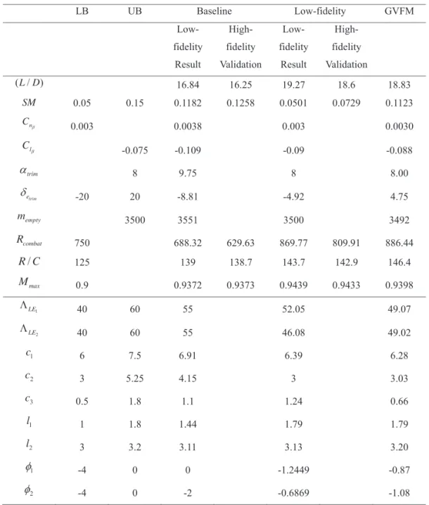
lift-to-Table 3. UCAV Optimization Results Table 3: UCAV Optimization Results

LB UB Baseline Low-fidelity GVFM Low-fidelity Result High-fidelity Validation Low-fidelity Result High-fidelity Validation ( / )L D 16.84 16.25 19.27 18.6 18.83 SM 0.05 0.15 0.1182 0.1258 0.0501 0.0729 0.1123 n C 0.003 0.0038 0.003 0.0030 l C_ _-0.075 _-0.109 _-0.09 _-0.088 trim



₈ _9.75 ₈ _8.00 trim e



_-20 ₂₀ _-8.81 _-4.92 _4.75 empty m ₃₅₀₀ ₃₅₅₁ ₃₅₀₀ ₃₄₉₂ combat R ₇₅₀ _688.32 _629.63 _869.77 _809.91 _886.44 / R C 125 139 138.7 143.7 142.9 146.4 max M _0.9 _0.9372 _0.9373 _0.9439 _0.9433 _0.9398 1 LE  ₄₀ ₆₀ ₅₅ _52.05 _49.07 2 LE  ₄₀ ₆₀ ₅₅ _46.08 _49.02 1 c ₆ _7.5 _6.91 _6.39 _6.28 2 c ₃ _5.25 _4.15 ₃ _3.03 3 c _0.5 _1.8 _1.1 _1.24 _0.66 1 l ₁ _1.8 _1.44 _1.79 _1.79 2 l ₃ _3.2 _3.11 _3.13 _3.20 1



_-4 ₀ ₀ _-1.2449 _-0.87 2



_-4 ₀ _-2 _-0.6869 _-1.08 (662~674)2017-141.indd 671 2018-01-05 오후 8:40:21

(11)

₆₇₂

drag ratio. The total number of design variables for the UCAV conceptual design problem is nine.

4. Results and Discussions

Both low-fidelity optimization and GVFM optimization were performed for comparison. Table 3 shows the results of the optimization. Fig. 14 shows the baseline and optimum UCAV configurations. In addition, the baseline and low-fidelity optimum configurations were analyzed using fidelity analysis. The result of the GVFM is equal to the high-fidelity function value by algorithm definition, so additional analysis is not required.

Comparison of the high- and low-fidelity analysis results for the baseline and the low-fidelity optimum configurations indicates that low-fidelity analysis overpredicts the value of (L/D) Aerodynamic analysis validation in section 2.2 exhibits similar behavior. A higher value of (L/D) leads to a 60 km longer combat radius. A static margin value is underpredicted by the low-fidelity analysis by a couple percent. The static margin of the baseline calculated using low-fidelity analysis is 11.8% versus 12.6% by CFD; similarly, the static margin is 5% versus 7.3% for the low-fidelity optimum.

Low-fidelity optimization terminated with the objective function improvement of approximately 14.4%. (L/D) increased from 16.84 to 19.27 in terms of the low-fidelity

46

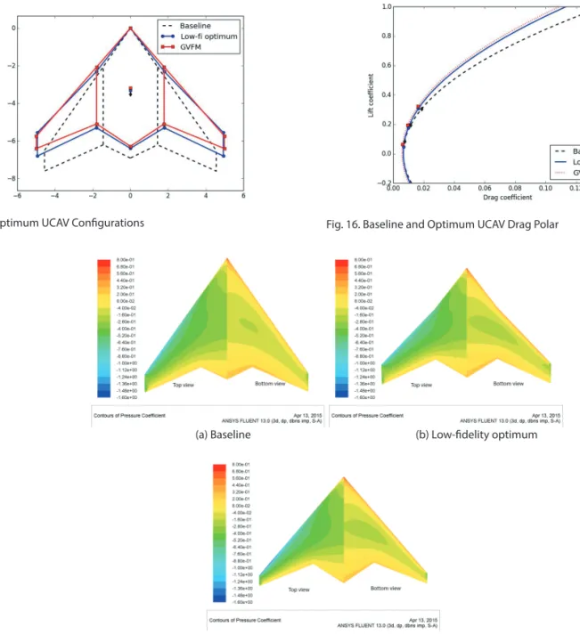
Fig. 14: Optimum UCAV Configurations

Fig. 14. Optimum UCAV Configurations

48

Fig. 16: Baseline and Optimum UCAV Drag Polar

Fig. 16. Baseline and Optimum UCAV Drag Polar

a) Baseline b) Low-fidelity optimum

c) Variable fidelity optimum Fig. 15: Surface Pressure Distribution

(c) Variable fidelity optimum Fig. 15. Surface Pressure Distribution

(a) Baseline (b) Low-fidelity optimum

(12)

673

http://ijass.org values. High-fidelity analysis of the optimum configuration

indicated a similar improvement of 14.4%, but the value of (L/D) predicted by CFD is lower. Variable fidelity optimization shows 16% objective function improvement compared to the baseline and 1.2% improvement compared to the low-fidelity optimum. These correlations can be observed in Fig. 16. The GVFM optimum has a lower (CD0),

while the induced drag coefficient is very similar to that of the low-fidelity optimum. Reduced (CD0) leads to faster

maximum speed, while smaller leading edge sweep angle leads slows it down. Combined these effects result in a very small increase of a maximum speed from Mach number of 0.9373 to 0.9398. Both of the optimum configurations have lower induced drag than the baseline. Classical performance analysis equations (e.g. Breguet equation) show that aircraft range is proportional to (L/D). Higher values of (L/D) and slightly lower empty mass led to a 9.4% longer combat radius compared to the low-fidelity optimum: 886 km versus 810 km. Variable fidelity optimization produced better results of optimization. Rate of climb is also highly affected by a lift-to-drag ratio as can be concluded from equations (2-4). Rate of climb increased from 138.7 to 142.9 and 146.4 m/s.

Regarding computational time, the GVFM algorithm evaluated the high-fidelity function 31 times until full convergence, including 25 times for the surrogate model initialization and 6 for the model refinement. A single run of high-fidelity analysis takes approximately 18 hours, and the single optimization loop takes approximately 1 hour. The total computational time required for UCAV design optimization using the variable fidelity algorithm is 23 full days on a desktop computer. This number is significantly lower than the number required for a pure high-fidelity optimization that can produce a result with similar accuracy. Pure low-fidelity optimization takes only 2 hours, but the level of accuracy is lower.

5. Conclusions

An integrated framework for the design and optimization of a flying wing UCAV was developed and validated. The framework is mainly based on low-fidelity analysis methods and empirical equations. An automated process for high-fidelity aerodynamic analysis of UCAV was developed and implemented in the design framework to increase the prediction accuracy of the analysis. The GVFM algorithm handles the interaction of high- and low-fidelity analysis disciplines for design optimization of a flying wing UCAV.

A flying wing UCAV MDO problem was formulated and successfully solved using two different approaches. The

first approach was optimization using a low-fidelity design framework. The second approach was variable fidelity optimization with MDO implementation of the GVFM algorithm. Variable fidelity optimization exhibited more design improvement with an acceptable computational cost compared to low-fidelity optimization.

Acknowledgement

This research was supported by Konkuk University Brain Pool 2017 and the International Research & Development Program of the National Research Foundation of Korea(NRF) funded by the Ministry of Science, ICT & Future Planning (Grant number: 2016K1A3A1A12953685).

References

[1] Hutchinson, J., “ Macrozanonia Cogn. and Alsomitra Roem”, Annals of Botany, Vol. 6, No. 1, 1942, pp. 95-102.

[2] Dunne, J. W., The Dunne Aeroplane, Flight, 1910, pp. 459-462.

[3] Green, W., Warplanes of the Third Reich, Macdonald and Jane’s Publishers Ltd, London, 1970.

[4] Northrop, J., “The Development of the All-Wing Aircraft”, The Aeronautical Journal, Vol. 51, No. 438, 1947, pp. 481-510.

[5] Bolsunovsky, A. L., Buzoverya, N. P., Gurevich, B. I., Denisov, V. E., Dunaevsky, A. I., Shkadov, L. M., Sonin, O. V., Udzhuhu, A. J. and Zhurihin, J. P., “Flying Wing - Problems and Decisions”, Aircraft Design, Vol. 4, No. 4, 2001, pp. 193-219.

[6] Kodiyalam, S. and Sobiezczanski-Sobieski, J., “Multidisciplinary Design Optimisation - Some Formal Methods, Framework Requirements, and Application to Vehicle Design”, International Journal of Vehicle Design, Vol. 25, 2001, pp. 3-22.

[7] Raymer, D., Aircraft Design: A Conceptual Approach (AIAA Education Series), American Institute of Aeronautics and Astronautics, Inc., Washington DC, 1992.

[8] Roskam, J., Airplane Design, DAR Corporation, Lawrence, Kansas, 1985.

[9] Torenbeek, E., Advanced Aircraft Design, John Wiley & Sons, Ltd., Netherlands, 2013.

[10] Torenbeek, E., “Fundamentals of Conceptual Design Optimization of Subsonic Transport Aircraft”, Delft University of Technology, Aerospace Engineering, 1980, Report No. LR-292.

[11] Prandtl, L., “Application of Modern Hydrodynamics to Aeronautics”, Technical Report, Washington, DC, National Advisory Committee for Aeronautics, 1923, Report No.

A Tailless UAV Multidisciplinary Design Optimization Using Global Variable Fidelity Modeling

662

Paper

A Tailless UAV Multidisciplinary Design Optimization Using Global

Variable Fidelity Modeling

Maxim Tyan*

Nhu Van Nguyen**

Jae-Woo Lee***

Abstract

1. Introduction

663

664

2. Integrated Analysis Framework for UAV

Design

2.1 Analysis Disciplines

665

666











































2.2 Variable Fidelity Aerodynamic Analysis

667

®

®

®

668









3. UCAV Design

3.1 Optimization Formulation

669



























670

3.2 Baseline Configuration and Design Variables









3.3 Framework Setup

671

3.4 Sensitivity Analysis









672

4. Results and Discussions

673

₆₆₄

₆₆₆

_®

_®

_®

₆₆₈

₆₇₀

₆₇₂