Deep Learning-Based Sustainable Data Center Energy Cost Minimization With Temporal MACRO/MICRO Scale Management

Received December 5, 2018, accepted December 8, 2018, date of publication December 19, 2018, date of current version January 16, 2019.

Digital Object Identifier 10.1109/ACCESS.2018.2888839

Deep Learning-Based Sustainable Data Center

Energy Cost Minimization With Temporal

MACRO/MICRO Scale Management

DONG-KI KANG , EUN-JU YANG, AND CHAN-HYUN YOUN, (Member, IEEE)

School of Electrical Engineering, Korea Advanced Institute of Science and Technology, Daejeon 34141, South Korea Corresponding author: Chan-Hyun Youn (chyoun@kaist.ac.kr)

This work was supported in part by the Cross-Ministry Giga KOREA Project grant through the Korean Government(MSIT) (Development of Mobile Edge Computing Platform Technology for URLLC Services) under Grant GK18P0400, and in part by the Institute for Information and Communications Technology Promotion (IITP) grant through the Korean Government(MSIT) (Service Mobility Support Distributed Cloud Technology) under Grant 2017-0-00294.

ABSTRACT Recently, distributed sustainable data centers based on renewable power generators have been deployed in order to efficiently reduce both the energy cost and carbon emission. Dynamic right-sizing (DRS) and frequency scaling (FS) have been considered as promising solutions to tune the computing capacity corresponding to the dynamic renewable power capacity. However, in existing works, the inaccurate power prediction and the uncoordinated decision making of DRS/FS still lead to low service quality and high energy cost. In this paper, we propose a novel joint optimization method for energy efficient distributed sustainable data centers. The proposed method adopts long short-term memory approach to improve the prediction accuracy of renewable power capacity for a long period, and unsupervised deep learning (DL) solver to resolve the coordinated DRS/FS optimization. Furthermore, we present the MACRO/MICRO (MAMI) time scale-based data center management technique to achieve both high energy efficiency and low wake-up transition overhead of DRS. To evaluate the proposed DL-based MAMI optimizer, we use the real trace data of renewable power capacity from the U.S. Measurement and Instrumentation Data Center. The experimental results demonstrate that our method reduces the energy cost by 25% compared with conventional metaheuristics while guaranteeing the service response delay requirement.

INDEX TERMS Energy efficiency, renewable energy sources, mathematical programming, unsupervised learning, economic forecasting.

I. INTRODUCTION

The modern geo-distributed sustainable data centers reduces the energy cost by using two renewable power sources, solar (or photovoltaic (PV)) power and the wind power [1]–[3]. In contrast to conventional grid power from coal and nuclear plants, sustainable power is (almost) free of fuel charge and does not generate the significant carbon emission. After the adoption of Paris climate assignment under the United Nations Framework Convention on Climate Change (UNFCCC) in Dec., 2015, countries encourage IaaS suppliers to operate their data centers based on renewable energy [4]. Facebook has depolyed multiple renewable energy generators in Los Lunas, New Mexico, Papillion, etc, to supply the energy requirement from geo-distributed data centers [5]. Apple has developed its own on-site renewable energy gen-erators of solar, water, wind, and biogas fuel cells. They have reduced CO2emission by 590,000 metric tons [6].

The exploitation of the on-site renewable power genera-tion should be carefully treated due to the associated inter-mittency and the uncertainty. The capacity of solar power depends on the solar radiation, and the wind power depends on the regional wind speed [7], [8]. Even in the same region, fluctuations in power capacity may arise due to changes in dynamic weather conditions [9]. The geo-distributed sustain-able data centers need the adaptive request dispatching (RD, i.e., mapping of data centers to requests) corresponding to dynamic renewable power capacity, to maximize their energy efficiency. For power capacity prediction, previous papers have proposed various methods such as nonlinear auto-regressive models with exogenous inputs (NARX) [10], esti-mated weighted moving average (EWMA) [11], and Kalman filter [12]. Even though such methods show good predictive performance however, they still exhibit low prediction accu-racy for irregular renewable power curves during long period.

Meanwhile, guaranteeing the service quality is also a criti-cal concern for sustainable data centers. There are two widely used methods for energy efficient data centers, dynamic right sizing (DRS) [13] and CPU frequency scaling (FS) [14], [15]. In the DRS, the number of powered-up servers is adjusted proportionally to the amount of incoming workloads. The DRS removes the static power consumption of idle servers, and results in both the energy saving and the high resource uti-lization. The FS indirectly tunes the power supply for running servers. The FS can adaptively control the CPU frequency of servers based on time-varying workloads and power capaci-ties and results in achieving the efficient dynamic power con-sumption. However, the coordinated management of DRS/FS is generally not easy to be designed due to following prob-lems. First, while FS overhead is negligible, the server wake-up transition overhead by DRS actuation is serious [13]. Too frequent DRS triggering causes non-negligible long server downtime, additional energy consumption, and cool-ing delay [9], [16], [17]. Second, many previous works have not considered both the DRS and FS as decision variables simultaneously since the coordination of DRS/FS makes the optimization problem non-convex [18]–[20]. Obviously, if we manage the DRS and FS separately, then we fail to achieve a better energy efficient data center in views of static and dynamic power consumption of servers.

In this paper, we propose the novel joint optimization algorithm for energy efficient sustainable data centers. Our work has following contributions.

• The objective of our optimization method is to find the optimal decision of DRS, FS, and RD for geo-distributed sustainable data centers in order to mini-mize energy cost while guaranteeing the service latency bound.

• We propose the MACRO/MICRO (MAMI) time scale

based management for energy efficient sustainable dis-tributed data centers. In MACRO time scale, the entire decision variables of DRS, FS, and RD are optimized simultaneously over the long time period. In MICRO time scale, given the fixed DRS decision, the decision of FS and RD are re-optimized corresponding to the work-load variation for the short-term period. This approach efficiently reduces the server wake-up transition over-heads caused by frequent DRS actuation.

• We adopt recurrent neural network (RNN) based long

short term memory (LSTM) method [21], which is the emerging artificial intelligent approach in order to improve the prediction accuracy for a long period. We present the LSTM input/output data structures dedi-cated to renewable power capacity prediction.

• We design the unsupervised deep learning (DL) solver

for non-convex optimization problem. Due to the benefit of unsupervised learning (i.e., not requiring labeling data), we can utilize both the actual and synthetic data to train the deep neural network (DNN) model [22]. The proposed DL based MAMI optimizer ensures the rapid output derivation once the DNN model is trained,

in contrast to conventional metaheuristics which require non-negligible re-compute time for each state.

In order to demonstrate the performance of the proposed DL based MAMI optimizer, we use real traces of solar radi-ation, outside air temperature, and wind speed at various geo-graphical locations, provided by the U.S. Measurement and Instrumentation Data Center (MIDC) [23]. Our MAMI optimizer integrating the LSTM predictor and the DL solver, outperforms conventional metaheuristics in views of both the energy cost and the service quaility ensurance of data cen-ters. Without violating the service latency bound, it reduces the energy cost about 25% compared to genetic algorithm (GA) [24]. Furthermore, the proposed optimizer requires the acceptable computation time (< 1s) for DRS/FS/RD decision making while the GA requires the undesirable time (> 1hr) for each decision making step.

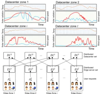
FIGURE 1. Fully connected structure of edge servers and geo-distributed sustainable data centers.

II. ENERGY COST MODEL FOR SUSTAINABLE DATA CENTERS WITH MULTIPLE EDGE SERVERS

We consider I sustainable data centers (DCs) with wind farms and solar panels, and J multiple edge servers. The edge servers (ESs) are scattered over multiple distributed edge zones which are populated areas (e.g., cities) to aggre-gate and transfer user requests to data centers [25], [26]. We assume that all the DCs and ESs are fully-connected each other [27]. This is shown in Fig.1. Let [x] = {1, · · · , x} denote the set of integer numbers which has x cardinality. Let Tcand K denote the considered continuous time length and the number of entire discrete time slots, respectively. The one time slot length is defined asδ = Tc

K. Then the discrete time slot indices k = 1, 2, · · · , K are mapped to countinous time intervals [0, δ), [δ, 2δ), · · · , [(K −1)δ, Kδ), respectively.

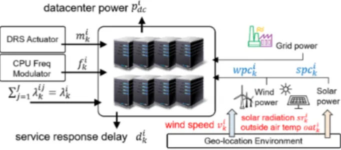
The geo-distributed sustainable DCs get their power supply from two main electricity facilities, grid power and renew-able power generators. Let sr_ki, oat_ki, and vi_k denote the weather condition variables; solar radiation, outside air tem-perature (OAT), and the wind speed in the i-th DC at time slot k, respectively. Let spci_kand wpci_kdenote the solar power and the wind power capacity based on the weather condition in the i-th DC at time slot k, respectively. Let mi_kand f_kidenote the number of powered-up servers and the CPU frequency value (the same value is set for all servers in DC) in the

i-th DC at time slot k. Let3j_k andλij_k denote the number of user requests entered to the j-th ES and the number of the dispatched requests from the j-th ES to the i-th DC at time slot k, respectively. Let λi_k = PJ_j=1λij

k denote the sum of user requests from entire edge servers. This structure is shown in Fig.2.

FIGURE 2. Dynamic Right Sizing (DRS) actuation, CPU Frequency Scaling (FS), and Request Dispatching (RD) for energy efficient sustainable data centers, with solar panels and wind farms.

A. RENEWABLE POWER CAPACITY MODEL 1) POWER CAPACITY OF SOLAR PANEL

The solar power is generated by sunlight through the solar panel converting sunlight into electrical power. The available solar power capacity spci_k is defined as follows [28]:

spci_k=ηi_Si_sri

k(1 − 0.005(oatki −25)), (1) where Siandηirepresent the size of panel area (m2) and the solar panel conversion efficiency (%), respectively. sr_ki and

oat_ki represent the amount of solar radiance (w/m2) and the outside air temperature (C), respectively; and they might be varied according to the dynamic weather condition.

2) POWER CAPACITY OF WIND FARM

The amount of electricity generated by wind farms depends on the regional wind speed and the blade characteristics. The approximated wind power capacity wpci_k is defined as follows [29]: wpci_k =              0, if vi_k < vci pr ∗ vi_k− vci vr− vci, if vci6 v i k6 vr pr, if vr 6 vik 6 vco 0, if vi_k > vco , (2)

where pr, vci, vr, vco are rated electrical power (w/m), cut-in wcut-ind speed (m/s), rated wind speed (m/s), and cut-off

wind speed (m/s), respectively. In particular, vci represents the wind speed at which the fan blades first start to rotate and produce the power (usually 3 − 5m/s) [7], [30]. vcorepresents the upper limit of the permissible wind speed to protect the turbine from the risk of damage due to strong wind speed (typically 25 − 30m/s).

B. DATA CENTER POWER CONSUMPTION MODEL

Let u and f denote the average CPU utilization and the CPU frequency of the arbitrary server in the data center, respec-tively. According to [31], the server power consumptoin p based on u and f can be approximated as follows:

p(f, u) = α3fu +α2f +α1u +α0. (3)

These power model coefficientsα0,α1,α2,α3 are derived

from curve-fitting methods. Note that the relationship u =λ_f holds where λ is the service arrival rate [31]. We assume that the user requests dispatched to the data center are evenly distributed to all the powered-up servers. That is, the average CPU utilization for single server in the i-th DC at time slot k is defined as ui_k = λ

i k

mi_kf_ki. Then, the total power consumption of the i-th DC at time slot k is defined as follows:

pi_dc(mi_k, f_ki, λ_ki) = mi_k(αi₃f_ki λ i k mi_kf_ki +αi 2fki+αi1 λi k mi_kf_ki +αi 0) =αi 3λ i k+α i 2m i kf i k +α i 1 λi k f_ki +αi 0m i k. (4)

Note that the static power consumptionαi₀mi_kcan be reduced only by powering down the idle servers via DRS actuation, since the adjustment of f_ki andλi_k affects only the dynamic power consumption.

C. DATA CENTER SERVICE RESPONSE LATENCY MODEL

For simplicity, we consider only the transactional workload as the type of user request in this paper. The performance of transactional workloads can be assesed by using the service response latency. We use M/M/m queueing model to model the average service response latency for each DC. The aver-age service response latency difor the i-th DC is defined as follows: di(mi_k, f_ki, λi_k) = PQ mi_kf_ki−λi k + 1 f_ki, (5)

where the first term of Eq.(5) denotes the average queue waiting time, and the second term denotes the average

ser-vice time. We simply assume that PQ = 1 which

repre-sents the probability of requests waiting in the queue refer to [3] and [32].

D. DATA CENTER ENERGY COST MINIMIZATION PROBLEM FORMULATION

Based on the Eq.(1)-(5), the energy cost model for the i-th DC at time slot k is defined as follows:

C_ki = di(mi_k, f_ki, λi_k) ∗ (pi_dc(mi_k, f_ki, λi_k) − spci_k− wpci_k)+, (6)

where (x)+_{=max(x, 0). For simplicity, the additional}

oper-ation cost for solar panels and wind farms is assumed to be free of charge in this paper. If spci_k+ wpci_{k > p}i_dc(mi_k, f_ki, λi_k), then the i-th DC is able to process the assigned user requests λi

k =

P

∀j∈[J ]λ

ij

kwith zero energy cost. Otherwise, the excess energy consumption is supported by the grid power generator, and the energy cost increases as the the amount of excess energy consumption increases.

The objective of this paper is to find optimal decision for DC energy cost minmiziation. The decision vector contains the number of powered-up servers m, the CPU frequency f, and the request dispatching mapλ. The predicted renewable

power capacity vectors spc, wpc and user requests 3 are

given over multiple time slots ∀k ∈ [K ]. We unfold these vectors as follows: • m = (m1₁, · · · , mI₁, m1₂, · · · , mI_K) ∈ RIK • f = (f1 1, · · · , f I 1, f 1 2, · · · , f I K) ∈ R IK • λ = (λ11 1 , λ 12 1 , · · · , λ 1J 1 , λ 21 1 , λ IJ 1, λ 11 2 , · · · , λ IJ K) ∈ RIJK • spc = (spc1 1, · · · , spcI1, spc12, · · · , spcIK) ∈ RIK • wpc = (wpc1 1, · · · , wpcI1, wpc12, · · · , wpcIK) ∈ RIK • 3 = (31 1, · · · , 3J1, 312, · · · , 3JK) ∈ RJK

Now, we formulate the problem for the energy cost minimiza-tion of distributed data centers as follows:

Problem 1 (Data Center Energy Cost Minimization):

min m,f,λC := K X k=1 I X i=1 C_ki + K X k=1 I X i=1 J X j=1 λij kt ij_ρij_{, (7)} subject to 1 mi_kf_ki−λi k + 1 f_ki 6 ¯d, ∀i ∈[I ], ∀k ∈ [K], (8) mi_kf_ki−λi_k > 0, ∀i ∈ [I], ∀k ∈ [K], (9) mi_{6 m}i_{k 6 m}i, ∀i ∈ [I], ∀k ∈ [K], (10) fi6 fki6 f i , ∀i ∈ [I], ∀k ∈ [K], (11) I X i=1 λij k =3 j k, ∀j ∈ [J], ∀k ∈ [K]. (12)

Here, tij andρij are the trasfer time and the link power consumption per data unit of user requests from j-th ES to

i-th DC, respectively. The constraint (8) indicates that the average service response latency can not exceed the prede-fined latency upper bound ¯d. The constraint (9) indicates that the number of user requests to dispatch can not exceed the available computing capacity of the destination DC. If it is violated, then the involved service response latency may be infinitely increased. The constraint (10) indicates that the number of powered-up servers should be adjusted within the number of total servers in the DC. The constraint (11) represents the available CPU frequency scaling range. The constraint (12) indicates that the user requests arrived at the certain ES should be entirely dispatched to distributed DCs.

Note that Problem1 has two main challenges. First, too frequent variation of m may aggravate the DRS wake-up transition overheads [13], [16]. This indicates that the DC

energy cost should be optimized with the minimum number of DRS triggering as possible. Second, the multiplication of

m and f in the constraints (8), (9) makes the Problem1 non-convex optimization. This prevents that the general non-convex optimizers solve the Problem1. To overcome these issues, we propose the novel optimization method in next section.

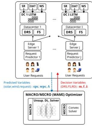
FIGURE 3. The structure of the proposed MACRO/MICRO (MAMI) optimizer, which consists of unsupervised deep learning (DL) solver (for MACRO time scale decision making) and convex solver (for MICRO scale decision making).

III. TEMPORAL MACRO/MICRO (MAMI) SCALE BASED DATA CENTER ENERGY COST OPTIMIZATION

In this section, we introduce our proposed deep learning (DL)

based MACRO/MICRO (MAMI) time scale optimizer. Fig.3

shows the structure of the proposed MAMI optimzer for geo-distributed sustainable data centers. The MAMI optimizer consists of unsupervised DL solver (for MACRO time scale decision making) and the convex solver (for MICRO time scale decision making). The long short term memory (LSTM) based predictor in each DC reports predicted renewable power capacity sequence to the MAMI optimizer. The request predictor in each ES reports predicted user request sequence to the MAMI optimizer. We show a detailed explanation of the DL solver and the LSTM predictor in section 4.

The MAMI optimizer differentiates the time scale for the variable m that is sensitive to switching overhead and the variables f andλ that are not sensitive to switching overhead. On the MACRO time scale, the MAMI optimizer fulfills the decision making for optimal m0, f, and λ. Here, m0 is the new decision vector defined for the shortened time slots

k0 = 1, · · · , K0_{, and it replaces the original decision vector} m. On the MICRO time scale, given fixed m0, the MAMI opti-mizer elaborately recalculates f andλ according to changes in solar power capacity, wind power capacity, and the user demands.

A. MACRO TIME SCALE DECISION MAKING

Let K0 denote the number of MACRO time slots such that

K0 < K. Let δ0 = q ·δ denote the MACRO time scale sam-pling interval where q is the positive integer number. Then, the MACRO time slot indices k0=0, 1, · · · , K0are mapped to 0, 1q, 2q, · · · , K. This relationship is shown in Fig.4. For the MACRO time scale decision making, we newly define

m0_=(m01 1, m 02 1, · · · , m 0I K0) ∈ RIK 0 instead of using m ∈ RIK_. Then we formulate the MACRO time scale DC energy cost minimization problem as follows:

FIGURE 4. MACRO/MICRO (MAMI) time scale control period.

Problem 2 (MACRO Time Scale Data Center Energy Cost Minimization): min m0_,f,λC 0_:= K0 X k0₌₁ q X k=1 I X i=1 C_ki0_,k+ K X k=1 I X i=1 J X j=1 λij ktijρij, (13) subject to 1 m0i_k0f_qki 0_+k−λi_qk0_+k + 1 f_qki 0_+k 6 ¯d, ∀i ∈[I ], ∀k ∈ [q], ∀k0∈[K0], (14) m0i_k0f_qki0_+k−λi_qk0_+k > 0, ∀i ∈ [I], ∀k ∈ [q], ∀k0∈[K0], (15) mi6 m0ik0 6 mi, ∀i ∈ [I], ∀k0∈[K0], (16) fi6 fqki 0_+k 6 f i , ∀i ∈ [I], ∀k ∈ [q], ∀k0∈[K0], (17) I X i=1 λij qk0_+k =3 j qk0_+k, ∀j ∈ [J], ∀k ∈ [q], ∀k0∈[K0], (18) where C_ki0_,k = di(m_k0i0, f_qki 0_+k, λi_qk0_+k) ∗ (pi_dc(m0i_k0, f_qki 0_+k, λi_qk0_+k) − spci_qk0_+k− wpci_qk0_+k) +_.

As the size of q increases, the dimensionality of m0 decreases. We can properly tune the DRS wake-up transition overhead by adjusting q. Note that replacing m using m0 has two advantageous points compared to naively adding the equality constraints to the Problem1. First, we decrease the

computation complexity by reducing the dimensionality of the decision vector. Second, we avoid the additional compu-tation burden for equality constraints.

Note that Problem 2 is the non-convex problem due to

the constraints (14), (15) which include the multiplication of decision variables m and f . In section 4, we show that our unsupervised DL solver efficiently resolves this non-convex problem.

B. MICRO TIME SCALE DECISION MAKING

The prediction of renewable power capacity does not always match with the actual data due to the intermittent and fluctuated properties of the weather condition (e.g., abrupt clouds and winds, drastic drop of temperature). Although the MACRO time scale based decision making efficiently reduces the DRS wake-up overheads however, it does not cope well with the renewable power capacity fluctuation immediately due to the long sampling period ofδ0.

FIGURE 5. MICRO time scale partial optimization for `f and `λ during interval [k =ζ, k = `K ] at k = ζ .

The goal of the MICRO time scale based decision making is to re-calculate the sophisticated frequency scaling/request dispatching, so as to complement the MACRO time scale management. Suppose that the the nontrivial prediction error for renewable power capacity is identified at k =ζ. In addi-tion, let spc0i_k and wpc0i_k denote the newly predicted solar and wind power capacity for time slot k, respectively. This is shown in Fig.5. The MAMI optimizer partially recalculates

f and λ corresponding to the renewaled prediction. To do

this, we define the MICRO time scale based DC energy cost minimization problem as follows:

Problem 3 (MICRO Time Scale Data Center Energy Cost Minimization): min `f,`λ;m0 C00:= ` K X k=ζ I X i=1 C<sub>k</sub>00i+ ` K X k=ζ I X i=1 J X j=1 λij kt ij_ρij_{, (19)} subject to 1 m00i_fi k −λ i k + 1 f_ki 6 ¯d, ∀i ∈[I ], k =ζ, ζ + 1, · · · , `K, (20) m00if_ki−λi_k > 0, ∀i ∈ [I],

k =ζ, ζ + 1, · · · , `K, (21) fi6 fki6 f

i

, ∀i ∈ [I], k = ζ, ζ + 1, · · · , `K, (22)

I X i=1 λij k =3 j k, ∀j ∈ [J], k =ζ, ζ + 1, · · · , `K, (23) where ` K = ζ + q − mod(ζ, q), m00i = m0i_k, k = dζ qe, `f = (f1 ζ, · · · , fζI, fζ +11 , · · · , f<sub>K</sub>`I) ∈ R I ·( `K −ζ)<sub>,</sub> ` λ = (λ11 ζ , · · · , λIJζ, λ11ζ+1, · · · , λIJ_K`) ∈ R IJ ·( `K −ζ )_,

C_k00i = di(m00i, f_ki, λi_k) ∗ (pi_dc(m00i, f_ki, λi_k) − spc0i_k− wpc0i_k)+. Here, mod(a, b) represents the remainder after a is divided by b. The number of powered-up servers is fixed as con-stant m00i derived from the optimal decision variable for the MACRO time scale problem. The MICRO time scale Problem3is resolved over the partial time slots from the cur-rent time slot index k =ζ to the next MACRO time slot index

k = `K. At every MACRO time slot, the MICRO time scale optimization can be iteratively conducted corresponding to the prediction error of renewable power capacity.

Contrary to the Problem2, the MICRO time scale Prob-lem3can be resolved by using the standard convex optimizer, since m00i is not the decision variable. Therefore, our DL solver only focuses on the MACRO time scale Problem2.

IV. UNSUPERVISED DEEP LEARNING SOLVER WITH THE LONG SHORT TERM MEMORY PREDICTOR

In this section, we explain the unsupervised deep learn-ing (DL) solver for non-convex MACRO time scale Prob-lem2. Furthermore, we introduce the long short term memory (LSTM) predictor to foresee the future renewable power capacity sequence.

A. LONG SHORT TERM MEMORY PREDICTOR FOR RENEWABLE POWER CAPACITY

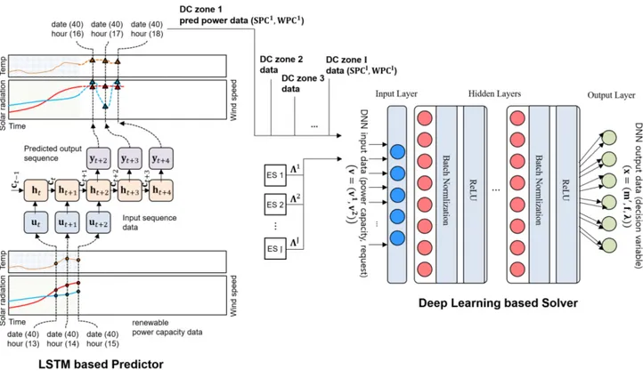
The structure of the LSTM network model is shown in the left part of Fig.6. The notations ut, ht, ct, yt denote input data block, hidden state block, cell state block, and output response block at training time step t, respectively. The output from hidden state htis derived from the non-linear hyperbolic tangent function tanh(x) = _coshsinh(x)_(x) = e2x−1

e2x₊₁. The backprop-agation of LSTM updates the weight parameters between each block based on the estimation error of output response sequence compared to the actual one. For details, see [33].

Obviously, the weather condition shows date and time-related periodical patterns (e.g., as shown in Fig.8). We define the date variable as the integer number dt ∈ [1, 365] (days) and the time variable as one within hr ∈ [1, 24] (hours). The input data sequence with length L is defined as follows:

(ui_t, ui_t+1, · · · , ui_t+L), (24) where

ui_t =(dt_ti, hr_ti, spci_t, wpci_t).

We also use L for the length of the predicted output respon-sce sequence. Then, the output response sequence is defined as follows:

(yi_t+L+1, yi_t+L+2, · · · , yi_t+2L), (25) where

yi_t =(spci_t, wpci_t).

After hiis updated, the predicted output response sequence (yi_t+L+1, · · · , yi_t+2L) is compared to the measured one (ˇyi_t+L+1, · · · , ˇyi_t+2L) where ˇyi_t+L+l is the measured output data at training time step t + L + l. The backpropagation is conducted based on the estimation error over the training time slots t, · · · , t + L, and entire network weight parameter matrices are updated. When closing the enough accuracy level, the training of LSTM network model is done.

Each DC conducts the inferencing for LSTM network model. At time slot k, all the DCs send the predicted renew-able power capacity sequence with L = K to the MAMI optimizer. If the non-negligible prediction error is identified

in i-th DC at certain time slot k = ζ, then the LSTM

based predictor re-trains the network model and the i-th DC sends the updated output response to the MAMI optimizer. The MICRO scale solver (i.e., convex optimizer) resolves the Problem3with updated prediction data of renewable power capacity.

B. UNSUPERVISED DEEP LEARNING BASED SOLVER FOR MACRO TIME SCALE OPTIMIZATION

The goal of our unsupervised DL solver is to find the (approx-imated) optimal decision vector for the non-convex MACRO time scale Problem2. To do this, we design the customized loss function for the DNN model training. The conventional loss function structures for supervised and unsupervised DL method are defined as follows [22], [34]:

E_Ns mb(w) = 1 Nmb Nmb X l=1 θ(ˇz(l), z(l)= DNN(v(l);w)). (26) E_Nu mb(w) = 1 Nmb Nmb X l=1 θ0 (z(l)= DNN(v(l);w)). (27) wt =wt−1−αt−1OwENmb(wt−1). (28) Here, w,θ, θ0_{, E}s Nmb, and E u

Nmbrepresent the network weight parameters, the supervised DNN loss function, unsupervised DNN loss function, average value of supervised DNN loss function, and the average value of unsupervised DNN loss function, respectively. Nmband DNN represent the minibatch size and the DNN model, respectively. v(l), ˇz(l), z(l)

repre-sent the input data, the label data corresponding to v(l), and

the estimated output data corresponding to v(l), respectively.

t and α represent the DNN training time slot index and

the learning rate, respectively. Note that Eq.(28) represents the gradient based formula for updating network weight parameters.

FIGURE 6. Proposed structure of unsupervised DL solver for MACRO Time Scale Problem and LSTM based renewable power capacity predictor.

In particular, we adopt the Eq.(27) to our proposed DL solver. In order to find the feasible solution for the MACRO time scale Problem 2, we add the simple penalty term8, which penalizes the violation of constraints (14) - (18). Consequently, we define our unsupervised DNN loss function as follows: θ0 (v;φ) = C0(x = DNN (v; w)) +8(x), (29) where 8(x) = K0 X k0₌₁ q X k=1 I X i=1 φd( 1 m0i_k0f_qki0_+k−λi_qk0_+k + 1 f_qki0_+k − ¯d)+ − K0 X k0₌₁ q X k=1 I X i=1 φposi(m0i k0f_qki 0_+k−λi_qk0_+k)− + K0 X k0₌₁ q X k=1 I X i=1 {φf(fi− f_qki0_+k)++φ_f(f_qki0_+k− f i )+} + K0 X k0₌₁ I X i=1 {φm(mi− mi_k0) +_+φm (mi_k0− mi) +_} + K X k=1 J X j=1 φλ| I X i=1 λij k−3 j k|,

andφ = (φd, φposi, φf, φ_f, φm, φm, φ_λ) is the set of penalty weight values for contraint violation. Here, (x)−=min(x, 0). The inferencing input data v and the inferencing output data x in our DNN loss function are defined as follows:

• v1 = (y1_t+L+1, · · · , yI_t+L+1, y1_t+L+2, · · · , yI_t+2L) ∈ R2IL • v2 = (31_t+L+1, · · · , 3_t+L+J ₁, 31_t+L+2, · · · , 3J_t+2L) ∈ RJL • v = (v1, v2) ∈ R2IL+JL • x = (m0, f, λ) ∈ RIK 0_{+IK +IJK}

For DNN training, the MAMI optimizer collects the his-torical data of renewable power capacity and user requests. If we do not have enough training dataset, then we can use the synthetic dataset which is randomly generated according to the predetermined distribution within the available ranges. The structure of the unsupervised DL solver is shown in the right part of Fig.6. The batch normalization technique [35] is applied to each hidden layer to avoid the gradient vanishing and exploding problems. We use the well-known rectified linear unit (ReLU) [36], [37] as the activation function for each neuron in our DNN model.

Algorithm 1 describes the MACRO time scale DC energy cost minimization procedures. The MAMI opti-mizer gathers the predicted renewable power capacity v1 = (y1_t+L+1, · · · , yI_t+2L) from LSTM predictor in each DC i = 1, · · · , I (line 01). The MAMI optimizer gathers the amount of predicted user requests v2 = (31_t+L+1, · · · , 3J_t+2L) from each ES j = 1, · · · , J (line 02). The input data vector v for DNN inferencing is generated resulting from integration of v1 and v2 (line 03). The decision variable

x = (m0, f, λ) is derived from inferencing the DNN model DNN(line 04).

Algorithm 1 MACRO Time Scale DC Energy Cost

Minimization

INPUT

Trained DNN model DNN with weight parameters w

OUTPUT

MACRO time scale optimal decision x = (m0, f, λ) 01 : gather predicted renewable power capacity from LSTM predictor in each DC 1, · · · , I,

v1_=(y1

t+L+1, · · · , yIt+2L)

02 : gather predicted user requests from edge servers (ESs),

v2=(31_t+L+1, · · · , 3J_t+2L)

03 : generate DNN input data vector v = (v1, v2) 04 : x = (m0_{, f, λ) ←− DNN(v; w)}

05 : return x

Algorithm 2 MICRO Time Scale DC Energy Cost

Minimization

INPUT

Starting MICRO time slot index, k =ζ

Number of powered-up servers m001, · · · , m00I by Eq.(24) Newly predicted solar power capacity

spc0i_k, k =ζ, · · · , `K, ∀i ∈ [I] Newly predicted wind power capacity

wpc0i_k, k =ζ, · · · , `K, ∀i ∈ [I]

OUTPUT

MICRO time scale partial optimal decision `f, `λ 01 : build C00by using Eq.(19)

02 : `f, `λ ←− solving MICRO time scale Problem3

03 : return `f, `λ

TABLE 1. Parameters for data center energy cost minimization problem.

Algorithm 2 describes the MICRO time scale DC energy cost minimization procedures. This algorithm is triggered whenever the significant prediction error for renewable power capacity is identified. The MICRO time scale cost function

C00 is built based on the error identification point k = ζ , the number of powered-up servers resulting from MACRO time scale optimization m001, · · · , m00I, and the newly pre-dicted solar/wind power capacity spc0i_k, wpc0i_k, k =ζ, · · · , `K, ∀i ∈ [I ] (line 01). The partial optimal solutions `f and `λ over k =ζ, · · · , `K are re-calculated via the standard convex optimizer (line 02).

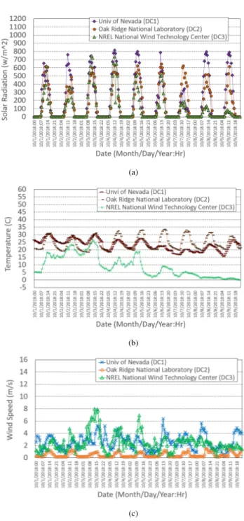
FIGURE 7. Curves of solar radiation, outside air temperatue, and wind speed during 2018.10.01-2018.10.08 (8days) at DC1 (Univ of Nevada), DC2 (Oak Ridge National Lab), and DC3 (NREL National Wind Technology Center, M2) [23]. (a) Actual solar radiation sr1, sr2_{, sr}3_(w/m2_). (b) Actual outside air temperature (OAT) oat1, oat2_{, oat}3_{(C ). (c) Actual} wind speed v1, v2_{, v}3_(m/s).

V. EXPERIMENTAL RESULTS

In our experiment, we deploy the physical machine with CPU i7-3770, gtx1080 (8GB), memory 16GB in order to train the LSTM model and the DNN model. We use CUDA 8.0 and cuDNN 5.0 [38] to accelerate the DNN training speed based on GPU. We use Keras 2.0.8 [39] APIs with Tensorflow framework 1.4 [40] in order to design the customized model structure of LSTM and DNN. To verify the performance of the proposed MAMI optimizer, we use real trace data of solar

FIGURE 8. Estimated curves of solar power capacity and wind power capacity during 2018.10.01-2018.10.08 (8days) at DC1 (Univ of Nevada), DC2 (Oak Ridge National Lab), and DC3 (NREL National Wind Technology Center, M2) [23]. (a) Available solar power capacity spc1, spc2_{, spc}3_{(kW ).} (b) Available wind power capacity wpc1, wpc2_{, wpc}3_{(kW ).}

TABLE 2. LSTM / DNN training parameters.

radiation, outside air temperature (OAT), and wind speed from geo-distributed DC regions in U.S [23]. We consider three regions: DC1-University of Nevada, Las Vegas (Par-adise, Nevada); DC2-Oak Ridge National Labotary (Eastern Tennessee); DC3-NREL National Wind Technology Center, M2 (Boulder, Colorado).

Fig.7and Fig.8show the curves of solar radiation, OAT, wind speed, solar power capacity, and wind power capac-ity during 2018.10.01-2018.10.08 (8days) at DC1 (Univ of Nevada), DC2 (Oak Ridge National Lab), and DC3

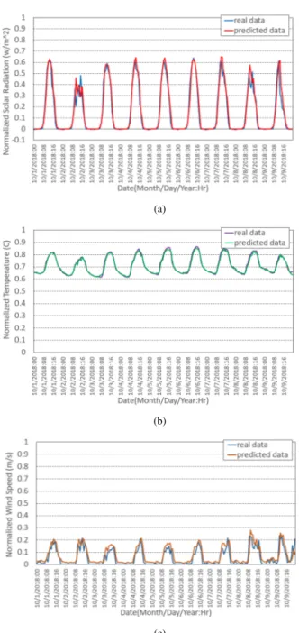
FIGURE 9. Prediction results for normalized solar radiation, outside air temperature (OAT), and wind speed during 2018.10.01-2018.10.08 (8days) at DC1 (Univ of Nevada) by the LSTM predictor. (a) Normalized solar radiation at DC1, sr1. (b) Normalized OAT at DC1, oat1. (c) Normalized wind speed at DC1, v1_.

(NREL National Wind Technology Center, M2). As shown in Fig.7-(a) and Fig.8-(a), the available solar power capac-ity strongly depends on the amount of solar radiation (the OAT influences are low). Similarly, the available wind power capacity is proportional to the wind speed as shown in Fig.7-(c) and Fig.8-(b). Note that the solar power capac-ity curve shows the regular patterns over time of the day. Contrary to DC1 and DC3, the available wind power capac-ity of DC2 is quite low due to the slow wind speed. This indicates that the accurate prediction for the solar power

FIGURE 10. Prediction results for normalized solar radiation, outside air temperature (OAT), and wind speed during 2018.10.01-2018.10.08 (8days) at DC2 (Oak Ridge National Laboratory) by the LSTM predictor. (a) Normalized solar radiation at DC2, sr2. (b) Normalized OAT at DC2, oat2. (c) Normalized wind speed at DC2, v2_.

capacity is relatively easy. Meanwhile, the curve of the wind power capacity depicts the irregular and intermittent patterns (Fig.8-(b)). This indicates that the prediction for the wind power capacity may show the lower accuracy than the solar power capacity.

The Table 1 presents the associated parameters for the energy cost minimization problem. We consider 3 geo-distributed DCs (DC1, DC2, and DC3) and 5 ESs. For sim-plicity, we assign the same bound of powered-up servers, bound of CPU frequency, and power coefficients for all the DCs. Every communication links between DCs and ESs

FIGURE 11. Prediction results for normalized solar radiation, outside air temperature (OAT), and wind speed during 2018.10.01-2018.10.08 (8days) at DC3 (NREL National Wind Technology Center, M2) by the LSTM predictor. (a) Normalized solar radiation at DC3, sr3. (b) Normalized OAT at DC3, oat3. (c) Normalized wind speed at DC3, v3.

have equal transfer time and power consumption per an user request. Note that we should define the proper penalty weight values for each constraint term in Eq.(30) to accurately find the feasiable solution. We assign the same penalty weight values (=103) to all the constraint terms except for request dispatching constraint (=105). This differentiated assignment attempts to avoid the rejection of entered user requests, as much as possible.

Table2presents the associated parameters for LSTM/DNN training. We retreive the training input dataset including hourly solar radiation, OAT and wind speed data from

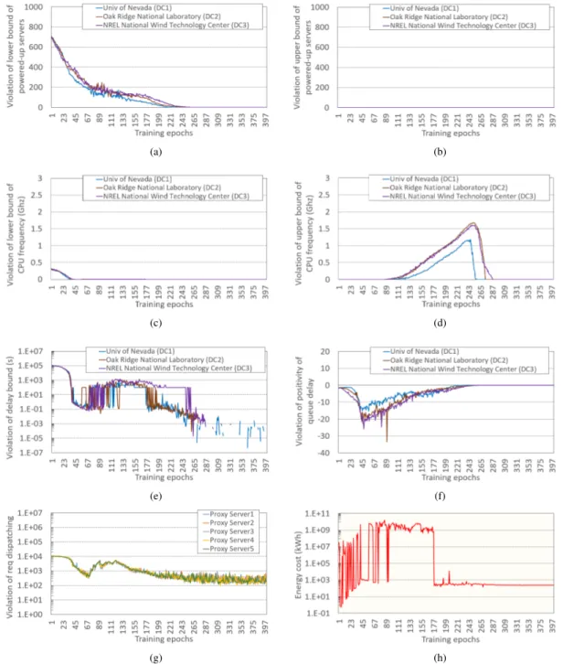
FIGURE 12. Experimental Results of DNN training progress with ¯d = 0.7sec for MACRO time scale problem optimization. The average degree of violation for all constraints involved in the MACRO time scale problem asymptotically decreases as the DNN training progresses. The average energy cost approaches the (approximated) optimal value 240kWh as the DNN training progresses. (a) Average violation of mi_{: (m}i−mi₎+_{. (b) Average violation of m}i_{: (m}i−mi)+_{. (c) Average violation} of fi: (fi−fi)+_{. (d) Average violation of f}i_{: (f}i−fi)+_{. (e) Average violation of ¯d : (d}i− ¯d )+_{. (f) Average violation of queue} delay positivity: (mi∗fi−λi)−_{. (g) Average violation of request dispatching: |}PI

i =1λij−3j|. (h) Average energy cost: C 0_.

DC1-DC3 during 2010.10.08 - 2018.10.09 (8years). The total number of data is about 7 × 105. We split the entire dataset into two groups, training dataset (6 × 105) and test dataset (9 × 104) for training validation. We set the maximum epochs for LSTM training as 100, however the early-stopping is possible when the LSTM loss function value reaches the predefined accuracy level. The associated SGD optimizer for LSTM is Adam, which exploits the adaptive estimates of

lower-order moments for stochastic gradient based optimiza-tion [41]. We adopt mean squared error (MSE) as the LSTM loss function [21], [42]. To foresee the hourly renewable power capacity for a half day, we set the LSTM timestep length as L = 12.

For DNN training, we use the training datset which is composed of historical renewable power capacity, and the his-torical amount of user requests. For renewable power capacity

FIGURE 13. Comparision results of proposed DL based MAMI optimizer and the rank based genetic algorithm [24] in temrs of energy cost (kWh) and the service response latency (sec). (a) Energy cost at 2018.10.10 (case1). (b) Energy cost at 2018.10.15 (case2). (c) Energy cost at 2018.10.20 (case3). (d) Service response latency with ¯d = 0.3s, 0.5s, 0.7s, 0.9s at 2018.10.10 (case1). (e) Service response latency with ¯d = 0.3s, 0.5s, 0.7s, 0.9s at 2018.10.15 (case2). (f) Service response latency with ¯d = 0.3s, 0.5s, 0.7s, 0.9s at 2018.10.20 (case3).

data, we adopt the same input data used for LSTM training. For user request data, we generate the synthetic raw dataset following the normal distribution with mean value 104and standard deviation 9 × 103. The dimension of the DNN input data is (2I + J ) ∗ K . The dimension of the DNN output data is I ∗ K0+ I ∗ K + J ∗ I ∗ K. Therefore, for I = 3, J = 5,

K0 =1, K = 12, the dimension of the input data is 132 and the dimension of the output data is 219. Our DNN model is simply composed of 1 fully connected hidden layers, 1 batch normalization layer [35] and 1 rectified linear unit (ReLU)

layer [36]. As described in section IV, we use Eq.(29) as the customized loss function for our unsupervised DL solver. The maximum epochs for DNN training is empirically set as the fixed value 400. Although the network depth level is not high, via the experimental results, we found that the trained DNN model draws the desirable solutions under var-ious renewable power capacity conditions (refer to Fig.13).

Fig. 9, 10, amd 11 show the prediction results for

normalized solar radiation, OAT, and wind speed during 2018.10.01-2018.10.08 (8days) at DC1-3 by using the LSTM

TABLE 3. Solar power capacity (kW), wind power capacity (kW), and amount of user requests (×103) at 06:00am - 05:00pm, 2018.10.10 (case1), 2018.10.15 (case2), and 2018.10.20 (case3) in DC1 (Univ of Nevada), DC2 (Oak Ridge National Lab), and DC3 (NREL National Wind Technology Center, M2).

based predictor. The amount of solar radiation shows the regular patterns over distributed DC regions, as shown in Fig.9-(a), Fig.10-(a), and Fig.11-(a). The OAT curves of DC1 and DC3 have somewhat irregular patterns (Fig.9-(b), Fig.11-(b)), while the DC2 has the regular OAT pattern (Fig.10-(b)). The wind speed curves of DC1 and DC3 also show aperiodic patterns (Fig.9-(c), Fig.11-(c)), while the DC2 has the periodic wind speed patterns (Fig.10-(c)). Note that the LSTM predictor achieves the high predic-tion accuracy under both the regular weather condipredic-tions and the irregular ones. However, for some control time points (e.g., 10/7/2018, 08:00 a.m in Fig.9-(a)), the transient predic-tion error for the renewable power capacity is identified. For such cases, the MICRO time scale management of the MAMI optimizer copes with the changing capacity patterns.

Fig.12 shows the results of DNN training progress for the customized loss function Eq.(29). The service response latency bound is ¯d = 0.7sec. The violation of box con-straints m, m, f , f is diminished along the progress of DNN training, as shown in Fig.12-(a), (b), (c), and (d). Inter-estingly, in Fig.12-(d), the violation of constraint for CPU frequency upper bound ¯f is consistently increased until the epoch = 250, and after then, it is drastically decreased.

This is because, as shown in Fig.12-(a), the DNN training is firstly performed aims to increase CPU frequency f , in order to mitigate the violation of the service response latency bound caused by the insufficient initial m. When m reaches a suf-ficient size at epoch = 250 however, the DNN training again performs weight parameter updating toward reducing the violation of CPU frequency upper bound. Fig.12-(e), (f), and (g) show the degrees of constraint violation for service response latnecy bound, the positivity of queue time, and the request dispatching, respectively. In Fig.12-(e) and (g), the associated constraint violation curves fall down during epoch = 0 − 60, increase during epoch = 60 − 120, and decrease consistently after epoch = 120. This is because, both the amount of the rejected requests and the service response latency are decreased, due to the increasing negativ-ity of queue time m ∗ f −λ (the excessive request dispatching to DCs) until epoch = 60, as shown in Fig.12-(f). However, after epoch = 60, updating the weight parameters in the direction of reducing the positivity violation of queue time is performed. Consequently, as shown in Fig.12-(h), our DL solver results in the network weight parameters which draw the minimized energy cost without any serious constraint violation.

In order to investigate the performance of our proposed DL based MAMI optimizer, we test three real cases based on renewable power capacity trace data during 12 hours: case1 (2018.10.10, 06:00 am - 05:00 pm at DC1-DC3); case2 (2018.10.15, 06:00 am - 05:00 pm at DC1-DC3); and case3 (2018.10.20, 06:00 am - 05:00 pm at DC1-DC3). The amount of user requests are randomly generated by using normal dis-tribution with average 104(reqs/sec) and standard deviation 9 × 103. The associated trace data is shown in Table3.

We adopt the rank based genetic algorithm (GA) [24] based DC management scheme as the conventional approach to compare with our proposed one. This scheme uses the adaptive penalty method by which the penalty weight values are iteratively updated during evolution phase according to the degree of constraint violation. It can be used to solve the constrained non-linear programming problem. For the GA scheme, we set the population size = 1000 in which each chromosome has 3177-bits binary genes. In addition, we set the mutation probabilty = 0.3, the selection pressure = 3 for roulette wheel procedure [9], and the evolution steps = 12000, respectively. Especially, we use the elitisim approach to guarantee the stable convergence to the optimal solution [43].

Fig.13-(a), (b) and (c) show the DC energy cost of the proposed MAMI optimizer and the rank based GA scheme. Note that the MAMI optimizer outperforms the GA scheme for every case regardless of the renewable power capacity condition. The MAMI optimizer achieves in average the reduction of energy cost about 25% compared to the GA scheme. The experimental results of service response latency

of DC1-DC3 for every case are shown in Fig.13 (d)-(f).

Note that the rank based GA scheme does not satisfy ser-vice response latency bound even for rather loosed values

¯

d = 0.7s, 0.9s. This indicates that the GA scheme is

not suitable for resolving the complex constrained problem. Contrary, even for the tight constraint value ¯d =0.3sec, the MAMI optimizer consistently satisfies the service response latency bound constraint for all cases. This indi-cates that the MAMI optimizer can generate the DNN weight parameters deriving feasible solution under all cases. We argue that the MAMI optimizer can be a promising alter-native for the conventional metaheuristics so as to solve the complex constrained optimization problem.

Furthermore, once the DNN model training is completed, the computation time for DNN inferencing is generally negli-gible. We found that the average inference time of our trained DNN model is less than 1s. Moreover, the DNN training time is acceptable. We found that the average training time for our DNN model is less than 30min. However, the rank based GA scheme needs the unacceptable re-computation time at each control time step. The average computation time required for the GA scheme appeared in Fig.13, is long than 10hr.

VI. CONCLUSION

In this paper, we proposed a deep learning (DL) based novel optimizer using long short term memory (LSTM) prediction

in order to achieve the energy cost efficient geo-distributed sustainable data centers. To the best of our knowledge, this is the first study to propose the data center energy cost optimization by using unsupervised DL method as the constrained non-convex problem solver. We proposed the temporal MACRO/MICRO (MAMI) time scale management technique in order to efficiently achieve the coordinated deci-sion making of dynamic right sizing (DRS) and the CPU frequency scaling (FS), and the request dispatching (RD). This technique minimizes the energy cost of data centers without the unacceptable DRS wake-up transition overhead. To demonstrate the performance of our proposed DL based MAMI optimizer, we used 7 ∗ 105real trace data of renew-able power capacity from U.S. Measurement and Instrumen-tation Data Center (MIDC). The adopted LSTM predictor showed the accurate prediction results for fluctuated solar and wind power capacity. The DL solver shows that it gradually approaches the feasible optimal solution for constrained non-convex optimization problem. Compared to the conventional rank based genetic algorithm (GA), on average, the proposed DL based MAMI optimizer reduces the DC energy cost about 25% for real trace data while gauranteeing the service quality requirement.

REFERENCES

[1] J. Qiu, J. Zhao, H. Yang, and Z. Y. Dong, ‘‘Optimal scheduling for prosumers in coupled transactive power and gas systems,’’ IEEE Trans.

Power Syst., vol. 33, no. 2, pp. 1970–1980, Mar. 2018.

[2] Y. Xiao, X. Wang, P. Pinson, and X. Wang, ‘‘A local energy market for electricity and hydrogen,’’ IEEE Trans. Power Syst., vol. 33, no. 4, pp. 3898–3908, Jul. 2018.

[3] D. Cheng, X. Zhou, Z. Ding, Y. Wang, and M. Ji, ‘‘Heterogeneity aware workload management in distributed sustainable datacenters,’’ IEEE Trans.

Parallel Distrib. Syst., p. 1, Aug. 2018, doi:10.1109/TPDS.2018.2865927.

[4] Adoption of the Paris Agreement, UNFCC, 2015. [Online]. Available: http://unfccc.int/resource/docs/2015/cop21/eng/l09.pdf

[5] Facebook. Adding Clean and Renewable Energy to the Grid. Accessed: Dec. 2018. [Online]. Available: https://sustainability.fb.com/clean-and-renewable-energy/

[6] Apple. To Ask Less of the Planet, We Ask More of Ourselves. Accessed: Dec. 2018. [Online]. Available: https://www.apple. com/lae/environment/climate-change/

[7] S. X. Chen, H. B. Gooi, and M. Q. Wang, ‘‘Sizing of energy storage for microgrids,’’ IEEE Trans. Smart Grid, vol. 3, no. 1, pp. 142–151, Mar. 2012.

[8] Q. Liu, Y. Ma, M. Alhussein, Y. Zhang, and L. Peng, ‘‘Green data center with IoT sensing and cloud-assisted smart temperature control system,’’

Comput. Netw., vol. 101, pp. 104–112, Jun. 2016.

[9] Y. Peng, D.-K. Kang, F. Al-Hazemi, and C.-H. Youn, ‘‘Energy and QoS aware resource allocation for heterogeneous sustainable cloud datacen-ters,’’ Opt. Switching Netw., vol. 23, pp. 225–240, Jan. 2017.

[10] H. Nazaripouya, B. Wang, Y. Wang, P. Chu, H. R. Pota, and R. Gadh, ‘‘Univariate time series prediction of solar power using a hybrid wavelet-ARMA-NARX prediction method,’’ in Proc. IEEE/PES Transmiss.

Dis-trib. Conf. Exposit. (T&D), May 2016, pp. 1–5.

[11] B. Aksanli, J. Venkatesh, L. Zhang, and T. Rosing, ‘‘Utilizing green energy prediction to schedule mixed batch and service jobs in data cen-ters,’’ in Proc. ACM 4th Workshop Power-Aware Comput. Syst., 2011, Art. no. 5.

[12] J. Zhang, G. Welch, G. Bishop, and Z. Huang, ‘‘A two-stage Kalman filter approach for robust and real-time power system state estimation,’’ IEEE

Trans. Sustainable Energy, vol. 5, no. 2, pp. 629–636, Apr. 2014. [13] M. Lin, A. Wierman, L. L. Andrew, and E. Thereska, ‘‘Dynamic

right-sizing for power-proportional data centers,’’ IEEE/ACM Trans. Netw., vol. 21, no. 5, pp. 1378–1391, Oct. 2013.

[14] X. Mei, X. Chu, H. Liu, Y.-W. Leung, and Z. Li, ‘‘Energy efficient real-time task scheduling on CPU-GPU hybrid clusters,’’ in Proc. INFOCOM

IEEE Conf. Comput. Commun., May 2017, pp. 1–9.

[15] D. Cheng, X. Zhou, P. Lama, M. Ji, and C. Jiang, ‘‘Energy efficiency aware task assignment with DVFS in heterogeneous Hadoop clusters,’’

IEEE Trans. Parallel Distrib. Syst., vol. 29, no. 1, pp. 70–82, Jan. 2018. [16] M. R. V. Kumar and S. Raghunathan, ‘‘Heterogeneity and thermal aware

adaptive heuristics for energy efficient consolidation of virtual machines in infrastructure clouds,’’ J. Comput. Syst. Sci., vol. 82, no. 2, pp. 191–212, 2016.

[17] Q. Fang, J. Wang, Q. Gong, and M. Song, ‘‘Thermal-aware energy man-agement of an HPC data center via two-time-scale control,’’ IEEE Trans.

Ind. Informat., vol. 13, no. 5, pp. 2260–2269, Oct. 2017.

[18] Z. Liu, M. Lin, A. Wierman, S. Low, and L. L. H. Andrew, ‘‘Greening geographical load balancing,’’ IEEE/ACM Trans. Netw., vol. 23, no. 2, pp. 657–671, Apr. 2015.

[19] D. Cheng, Y. Guo, C. Jiang, and X. Zhou, ‘‘Self-tuning batching with DVFS for performance improvement and energy efficiency in Internet servers,’’ ACM Trans. Auto. Adapt. Syst., vol. 10, no. 1, 2015, Art. no. 6. [20] Z. Liu et al., ‘‘Renewable and cooling aware workload management for

sustainable data centers,’’ ACM SIGMETRICS Perform. Eval. Rev., vol. 40, no. 1, pp. 175–186, 2012.

[21] K. Greff, R. K. Srivastava, J. Koutník, B. R. Steunebrink, and J. Schmidhu-ber, ‘‘LSTM: A search space odyssey,’’ IEEE Trans. Neural Netw. Learn.

Syst., vol. 28, no. 10, pp. 2222–2232, Oct. 2017.

[22] I. Goodfellow, Y. Bengio, A. Courville, and Y. Bengio, Deep Learning, vol. 1. Cambridge, MA, USA: MIT Press, 2016.

[23] Measurement and Instrumentation Data Center (MIDC), Accessed: Dec. 2018. [Online]. Available: https://midcdmz.nrel.gov/

[24] R. de Paula Garcia, B. S. L. P. de Lima, A. C. de Castro Lemonge, and B. P. Jacob, ‘‘A rank-based constraint handling technique for engineering design optimization problems solved by genetic algorithms,’’ Comput.

Struct., vol. 187, pp. 77–87, Jul. 2017.

[25] L. Peng, A. R. Dhaini, and P.-H. Ho, ‘‘Toward integrated Cloud–Fog networks for efficient IoT provisioning: Key challenges and solutions,’’

Future Gener. Comput. Syst., vol. 88, pp. 606–613, Nov. 2018.

[26] L. Peng, ‘‘On the future integrated datacenter networks: Designs, opera-tions, and soluopera-tions,’’ Opt. Switching Netw., vol. 19, pp. 58–65, Jan. 2016. [27] Y. Zhang, M. Chen, N. Guizani, D. Wu, and V. C. Leung, ‘‘SOVCAN: Safety-oriented vehicular controller area network,’’ IEEE Commun. Mag., vol. 55, no. 8, pp. 94–99, 2017.

[28] A. Yona, T. Senjyu, A. Y. Saber, T. Funabashi, H. Sekine, and C.-H. Kim, ‘‘Application of neural network to 24-hour-ahead generating power fore-casting for PV system,’’ in Proc. IEEE Power Energy Soc. Gen.

Meeting-Conversion Del. Electr. Energy 21st Century, 2008, pp. 1–6.

[29] D. T. Nguyen and L. B. Le, ‘‘Optimal bidding strategy for microgrids con-sidering renewable energy and building thermal dynamics,’’ IEEE Trans.

Smart Grid, vol. 5, no. 4, pp. 1608–1620, Jul. 2014.

[30] J. Aho et al., ‘‘A tutorial of wind turbine control for supporting grid frequency through active power control,’’ in Proc. IEEE Amer. Control

Conf. (ACC), Jun. 2012, pp. 3120–3131.

[31] T. Horvath and K. Skadron, ‘‘Multi-mode energy management for multi-tier server clusters,’’ in Proc. IEEE Int. Conf. Parallel Archit. Compilation

Techn. (PACT), Oct. 2008, pp. 270–279.

[32] Y. Zhang, Y. Wang, and X. Wang, ‘‘Greenware: Greening cloud-scale data centers to maximize the use of renewable energy,’’ in Proc.

ACM/IFIP/USENIX Int. Conf. Distrib. Syst. Platforms Open Distrib. Pro-cess.Berlin, Germany: Springer, 2011, pp. 143–164.

[33] W. Zhu et al., ‘‘Co-occurrence feature learning for skeleton based action recognition using regularized deep LSTM networks,’’ in Proc. AAAI, vol. 2, no. 5, 2016, p. 6.

[34] M. Chen, X. Shi, Y. Zhang, D. Wu, and M. Guizani, ‘‘Deep fea-tures learning for medical image analysis with convolutional autoen-coder neural network,’’ IEEE Trans. Big Data, p. 1, Jun. 2017, doi:

10.1109/TBDATA.2017.2717439.

[35] S. Ioffe and C. Szegedy, ‘‘Batch normalization: Accelerating deep network training by reducing internal covariate shift,’’ in Proc. Int. Conf. Mach.

Learn., 2015, pp. 448–456.

[36] V. Nair and G. E. Hinton, ‘‘Rectified linear units improve restricted Boltz-mann machines,’’ in Proc. 27th Int. Conf. Mach. Learn. (ICML), 2010, pp. 807–814.

[37] S. Wan, Y. Liang, Y. Zhang, and M. Guizani, ‘‘Deep multi-layer perceptron classifier for behavior analysis to estimate parkinson’s disease severity using smartphones,’’ IEEE Access, vol. 6, pp. 36825–36833, 2018.

[38] NVIDIA Developer. Accessed: Dec. 2018. [Online]. Available: https://developer.nvidia.com/

[39] Keras: The Python Deep Learning Library. Accessed: Dec. 2018. [Online]. Available: https://keras.io/

[40] TensorFlow: An Open Source Machine Learning Library for Research and

Production. [Online]. Available: https://www.tensorflow.org/

[41] D. P. Kingma and J. Ba. (2014). ‘‘Adam: A method for stochastic optimiza-tion.’’ [Online]. Available: https://arxiv.org/abs/1412.6980

[42] S. Xiao, H. Yu, Y. Wu, Z. Peng, and Y. Zhang, ‘‘Self-evolving trading strategy integrating Internet of Things and big data,’’ IEEE Internet Things

J., vol. 5, no. 4, pp. 2518–2525, Aug. 2018.

[43] K. Deb, A. Pratap, S. Agarwal, and T. Meyarivan, ‘‘A fast and elitist multiobjective genetic algorithm: NSGA-II,’’ IEEE Trans. Evol. Comput., vol. 6, no. 2, pp. 182–197, Apr. 2002.

DONG-KI KANG received the M.S. degree in computer engineering from Chonbuk National University, Jeonju, South Korea, in 2011. He is currently pursuing the Ph.D. degree in electrical engineering with the Korea Advanced Institute of Science and Technology, Daejeon, South Korea. His research interests include cloud computing, deep learning, and GPU power control.

EUN-JU YANG received the M.S. degree in electrical engineering from the Korea Advanced Institute of Science and Technology, Daejeon, South Korea, in 2018, where she is currently pursu-ing the Ph.D. degree in electrical engineerpursu-ing. Her research interests include deep learning, machine learning distributed processing, and multi-access edge computing.

CHAN-HYUN YOUN (S’84–M’87) received the B.Sc. and M.Sc. degrees in electronics engineer-ing from Kyungpook National University, Daegu, South Korea, in 1981 and 1985, respectively, and the Ph.D. degree in electrical and communica-tions engineering from Tohoku University, Sendai, Japan, in 1994. Before joining the University, from 1986 to 1997, he was the Leader of the High-Speed Networking Team, KT Telecommunications Net-work Research Laboratories, where he had been involved in the research and developments of centralized switching mainte-nance system, maintemainte-nance and operation system for various ESS’s system, high-speed networking, and ATM network testbed. Since 1997, he has been a Professor with the School of Electrical Engineering, Korea Advanced Institute of Science and Technology (KAIST), Daejeon, South Korea. He was an Associate Vice-President of office of planning and budgets in KAIST from 2013 to 2017. He has authored a book on Cloud Broker and Cloudlet

for Workflow Scheduling(Springer, 2017). His research interests include distributed high performance computing systems, cloud computing systems, edge computing systems, deep learning framework, and others. He received the Best Paper Award from CloudComp 2014. He was a General Chair for the 6th EAI International Conference on Cloud Computing, KAIST, in 2015. He was a Guest Editor of the IEEE WIRELESSCOMMUNICATIONSin 2016.