저작자표시-비영리-변경금지 2.0 대한민국 이용자는 아래의 조건을 따르는 경우에 한하여 자유롭게 l 이 저작물을 복제, 배포, 전송, 전시, 공연 및 방송할 수 있습니다. 다음과 같은 조건을 따라야 합니다: l 귀하는, 이 저작물의 재이용이나 배포의 경우, 이 저작물에 적용된 이용허락조건 을 명확하게 나타내어야 합니다. l 저작권자로부터 별도의 허가를 받으면 이러한 조건들은 적용되지 않습니다. 저작권법에 따른 이용자의 권리는 위의 내용에 의하여 영향을 받지 않습니다. 이것은 이용허락규약(Legal Code)을 이해하기 쉽게 요약한 것입니다. Disclaimer 저작자표시. 귀하는 원저작자를 표시하여야 합니다. 비영리. 귀하는 이 저작물을 영리 목적으로 이용할 수 없습니다. 변경금지. 귀하는 이 저작물을 개작, 변형 또는 가공할 수 없습니다.
이
학 석 사 학 위 논 문
Relative Contribution of Different Plant
Functional Types to Growing Season Gross
Primary Productivity Interannual Variation
in Alaska
식생유형이
알라스카 총 1차 생산성의 연간변화에 미치는
상대적인
기여
February 2018
서울대학교 대학원
협동과정 농림기상학
Jane Lee
RELATIVE CONTRIBTUION OF DIFFERENT PLANT
FUNCTIONAL TYPES TO GROWING SEASON GROSS
PRAIMARY PRODUCTIVITY INTERANNUAL VARIATION
IN ALASKA
UNDER THE SUPERVISION OF PROFESSOR YOUNGYREL RYU
SUBMITTED TO THE FACULTY OF THE GRADUATE SCHOOL OF SEOUL NATIONAL UNIVERSITY
BY JANE LEE
INTERDISCIPLINARY PROGRAM IN AGRICULTURAL AND FOREST METEOROLOGY
DECEMBER 2017
APPROVED AS A QUALIFIED THESIS OF JANE LEE
FOR THE DEGREE OF MASTER OF SCIENCE IN AGRICULTURAL AND FOREST METEOROLOGY
BY COMMITTEE MEMBERS JANUARY 2018
CHAIRMAN _____________________________ Hyun Seok Kim, Ph.D.
VICE-CHAIRMAN _____________________________ Youngyrel Ryu, Ph.D.
MEMBER _____________________________ Sang Jong Park, Ph.D.
i
ABSTRACT
Relative Contribution of Different Plant Functional Types to Growing
Season Gross Primary Productivity Interannual Variation in Alaska
Jane Lee Interdisciplinary Program in Agricultural and Forest Meteorology The Graduate School of Seoul National University
Vegetation in the high latitude ecosystem is most responsive to climate variables, leading to high year to year variability of gross primary productivity (GPP). Therefore, understanding the spatiotemporal patterns of GPP and how climate variables drive its interannual variability (IAV) is important to account for their present and future status. In this study, we examine the spatiotemporal patterns of Alaskan GPP and further investigate how their relation to climate drivers. We use GPP derived from four different approaches, a process-based approach (Breathing Earth System Simulator), a semi-empirical approach (Moderate Resolution Spectroradiometer 17A2) and the machine-learning approaches (Support Vector Regression and FLUXCOM). Model evaluation with eddy covariance data from 17 sites showed that the models explained 65% to 85% of the monthly variation with relative bias ranging from -22% to 33%. Model performance was better in the boreal forest compared to tundra and fire disturbed ecosystems. The spatial and temporal variation of GPP in the models displayed a consistent pattern, where the deciduous broadleaf forest showed the highest variability of GPP IAV by 14%, followed by fire and evergreen forest (13%) and then tundra (10%). Tundra accounted for the largest fraction of IAV of GPP with 55%, exceeding evergreen needleleaf forest (38%), deciduous broadleaf forest (7%) and areas that had been disturbed by fire (0.8%). GPP in tundra has the smallest variation among the PFTs. 68% of Alaska is tundra which led to the largest contribution to the IAV of GPP. The IAV of GPP from 2001 to 2011 had a similar pattern to the IAV of both air temperature and radiation, where warmer years had a larger GPP anomaly compared to the colder years. Therefore, warming and cooling as a result of climate change could significantly impact the IAV of land-atmosphere interaction of carbon dioxide.
Keywords: interannual variation, gross primary productivity, air temperature, radiation, precipitation, Alaska
ii
TABLE OF CONTENTS
ABSTRACT... i
TABLE OF CONTENTS ... ii
LIST OF TABLE ... iii
LIST OF FIGURES ... iv
1. Introduction ... 5
2. Material and Method ... 9
2.1 Study Region ... 9
2.2 Flux Tower Data ... 10
2.3 Satellite-based GPP Datasets ... 13
2.4 Dataset of climate variables ... 18
2.5 Landcover map ... 19
2.6 Evaluation and analysis of GPP ... 20
3. Results... 24
3.1 Evaluation of Models against flux tower data ... 24
3.2 IAV of GPP ... 27
3.3 Relationship between IAV of GPP and Climate Variables ... 35
4. Discussion ... 41
4.1 Model Performance across different PFTs ... 41
4.2 IAV of GPP ... 43
4.3 Controlling factors in IAV of GPP ... 45
5. Conclusion ... 47
iii
Abstract in Korean ... 57 Acknowledgement ... 58
LIST OF TABLE
Table 1. Flux tower site information ... 11 Table 2. Summary of Model Approach and MODIS input forcing data ... 17 Table 3. Evaluation of BESS, MODIS, SVR and FLXUCOM………24
iv
LIST OF FIGURES
Figure 1 Plant functional type map of Alaska... 10
Figure 2 Evaluation of modeled GPP at a monthly time scale. ... 27
Figure 3 The Relative standard deviation (%) of GPP IAV . ... 29
Figure 4 Averaged relative standard deviation of GPP IAV. ... 30
Figure 5 Relative contribution (%) of each grid cell to GPP IAV. ... 32
Figure 6 (a) The sum of relative contribution of GPP IAV for each PFT, and the (b) the IAV of GPP from 2001 to 2011 in Alaska. ... 33
Figure 7 Relative contribution of PFT to GPP ... 35
Figure 8 RGB composite of climatic drivers. ... 37
Figure 9 The mean and sum of relative contribution to GPP IAV. ... 39
5
1. Introduction
The Arctic ecosystem, characterized by low temperatures and short growing seasons, plays a unique role in the land-atmosphere exchange of carbon dioxide (Bliss et al., 1973, McGuire et al., 2006, Schuur et al., 2015). During the Holocene (approximately 11,700 years ago), the arctic system was a net carbon sink (Oechel
et al., 1993, Ping et al., 2008), with pervasive cold temperatures limiting the decay
of soil organic carbon, resulting in the accumulation of carbon above and beneath the permafrost in peatlands over centuries to a millennia (Strauss et al., 2013). Substantial warming, induced by anthropogenic fossil fuel emission, in the high latitudes is occurring faster compared to the rest of the globe (Bekryaev et al., 2010, Bieniek and Walsh 2017). This is causing frozen ground to thaw, exposing large quantities of organic carbon to soil microbes for decomposition, leading to the release of greenhouse gases into the atmosphere that could increase the rate of global warming (Nauta et al., 2014, Schuur et al., 2015). Warming is also lengthening growing seasons allowing vegetation productivity to increase (Jeong et
al., 2011, Guay et al., 2014, Park et al., 2016), or stimulating respiration depending
on plant functional types (Piao et al., 2008, Euskirchen et al., 2016, Commane et
al., 2017), affecting the carbon balance of the ecosystem. Such changes in the arctic
6 et al., 2005, Zeng et al., 2017).
Changes in gross primary productivity (GPP) across different plant functional types (PFT) are non-linear in the high latitudes as they are affected by warming in the recent decades (Park et al., 2015). GPP in the cooler high latitudes show an increase, due to warming, while the warmer lower latitudes show a decline (Mekonnen et al., 2016). Ueyama et al., (2014) reveals that a black spruce forest in the Interior of Alaska shifted from a CO2 sink to source as autumn air temperatures
increased over 9 years. Satellite observations also show that the boreal forests are “browning” whereas arctic tundra continues “greening.” (Beck and Goetz 2012, Xu
et al., 2013). The response of vegetation to climate drivers can change (Piao et al.,
2014, Wang et al., 2015, Piao et al., 2017), therefore, it is important to understand the spatiotemporal patterns of GPP and how climate variables drive its year to year variability to account for their present and future status.
The pattern of GPP interannual variability (IAV) is determined by climate variables, vegetation types and their spatial distribution (Zhang et al., 2016, Zhou
et al., 2017). GPP in tundra ecosystems is controlled by environmental factors such
as, the time of snowfall or snowmelt and leaf out and leaf fall, which determines growing season length (Euskirchen et al., 2012, Ueyama et al., 2013). In evergreen needleleaf forests (ENF), GPP is detected when the environment becomes favorable as their photosynthetic apparatus are already assembled (Goulden et al., 1998, Welp
7
et al., 2007). GPP in deciduous broadleaf forests (DBF) are more sensitive to spring
temperatures and lags compared to ENF as leaf develops, but after leaf-out they compensate for the late start by higher assimilation rates during the middle of the growing season (Black et al., 2000, McGuire et al., 2006, Welp et al., 2007, Zhang
et al., 2017). Forests disturbed by fire have smaller GPP than undisturbed forests,
but with varying magnitude of GPP depending on the rate of recovery, which increases the rate of carbon dioxide IAV in the northern hemisphere (Randerson et
al., 2006, Yi et al., 2013). In short, the larger variation of GPP in ENF is modulated
by physiology rather than phenology. In contrast, both the physiology and phenology of DBF, tundra and disturbed sites explains GPP IAV. Previous studies have intensively focused on how the structure of canopy, leaf-on and leaf-fall of different PFTs affect GPP responses to climate variability (Yuan et al., 2009, Mekonnen et al., 2016), but we still lack a comprehensive understanding of how different PFTs contribute to GPP IAV in Alaska.
Gross primary productivity can be derived from a regional to global scale through combining various approaches, such as the process-based, semi-empirical or machine learning, with remote sensing products and meteorological datasets. Process-based approaches employ biophysical theories to provide insight to the underlying mechanisms of environmental change on vegetation activity (Ryu et al., 2011, Jiang and Ryu 2016). Semi-empirical approaches use algorithms with
8
empirical constraints to estimate the desired variable such as light use efficiency (Running et al., 2004). Machine-learning approaches use exiting data to train statistical models, and apply the model to a larger area with the explorative variables (Ueyama et al., 2013, Tramontana et al., 2016). Major model comparison projects demonstrate that there are large variations within model estimations of GPP due to varying forcing data, model structure and parameterization, yet an ensemble of models can reduce bias of estimates from models (Cramer et al., 1999, Sitch et al., 2007, Huntzinger et al., 2013, Piao et al., 2013, Ito et al., 2016). Therefore, we use the products of these different approaches to analyze the spatial and temporal patterns of GPP interannual variability and its response to with climate variability. Here, our goal is to quantify the spatial and temporal patterns of GPP IAV in Alaska growing season. To achieve our goal, we test the performance of four GPP models against 17 flux tower data from different PFTs. Then we investigate the spatial and temporal patterns of GPP, quantifying the relative contributions of PFTs to GPP IAV in Alaska. Finally, we examine the relationship of GPP with climate variables at a regional scale.
9
2. Material and Method 2.1 Study Region
We defined our study region, Alaska, excluding the southeastern Alaskan Panhandle, with latitudes and longitudes of 72˚N to 52˚N and 170˚W to 140˚W, respectively. Alaska can be mainly characterized as the Arctic and interior Alaska, based on climate, vegetation type and permafrost distribution. The Arctic is found north of the Brooks Range, covered by tundra vegetation with continuous permafrost. The interior of Alaska is located north of the Alaska Range and south of the Brooks Range, which is mostly boreal forest underlying discontinuous permafrost. The annual mean air temperature is -12˚C and annual precipitation is 100 to 130 mm yr-1 in Alaska.
10 Figure 1 Plant functional type map of Alaska
2.2 Flux Tower Data
Eddy covariance flux data of GPP gathered from 21 sites in Alaska was used in courtesy of Ueyama et al., (2013) for model evaluation. The tower sites are situated in various representative ecosystems of Alaska (Figure 1): wet sedge tundra (CMS, BEC and IMW), moist tussock tundra (ATQ, IVO, IMT and ARU), black spruce forest (PFA, UAF and DLS), Aspen forest (DLA) and burned black spruce forest (CRF, PFR and DLB). The winter and growing season data was present for 13 of the sites, and only the growing season was available for 7 of the sites. Our study period is from 2001 to 2011, where 17 of the 21 sites were available for
11
evaluating GPP from models. Table 1 presents detailed information of each site. All data were processed with a standardized gap filling, quality control and flux-partitioning procedures. The quality control of the eddy covariance data was primarily conducted by site mangers. Ueyama et al., (2013) manually removed the outliers and spike-like data and applied a look-up table and nonlinear regression for gap filling and flux partitioning methods. If a lookup table was not applicable, then the nonlinear regression was used. One precaution about partitioning GPP and Ecosystem Respiration (ER) from Net Ecosystem Exchange (NEE) is that nighttime data was used, where nighttime is almost nil in summer. Nighttime data is limited in the Arctic, and thus the performance of respiration models may be less accurate compared to other regions. These flux data were used to upscale from a site level to a regional scale in Alaska with the Support Vector Regression Model from the period of 2000 to 2011 (Ueyama et al., 2013).
12
Site Code Lat (° N)
Lon (°
W) Type (PFT) Vegetation Years
Mean Annual Temperatur e1 (° C) Mean Annual Precipitation2 (mm) Reference University of Alaska Fairbanks (UAF) 64.87 -147.86 Black Spruce Forest (ENF) 2003-2014 -1.83 309.12 (Iwata et al., 2012); (Ueyama et al., 2014) Poker Flat Research Range (PFR) 65.12 -147.43 Burned Forest (ENF) 2009-2012 -1.94 308.36 (Iwata et al., 2011) Poker Flat Research Range (PFA) 65.12 -147.49 Black Spruce Forest (ENF) 2011-2014 -1.94 308.36 (Nakai et al., 2013) Bonanza Creek LTER (BNB) 64.69 -148.32 Black Spruce Forest (ENF) 2010-2013 -1.94 308.36 (Euskirchen et al., 2012) Delta Junction (DLS) 63.92 -145.75 Black Spruce Forest (ENF) 2003-2005 -1.67 295.15 (Randerson et al., 2006); (Welp et al., 2007) Delta Junction (DLA) 63.92 -145.37 Aspen Forest (DBF) 2002-2004 -1.67 295.15 (Randerson et al., 2006); (Welp et al., 2007) Delta Junction (DLB) 63.89 -145.74 Burned Forest (ENF) 2002-2004 -1.67 295.15 (Randerson et al., 2006); (Welp et al., 2007) Anaktuvuk River (ARS) 68.98 -150.28 Severely Burned Tundra 2008-2010 -11.00 122.17 (Rocha and Shaver 2011) Anaktuvuk River (ARM) 68.95 -150.21 Moderately Burned Tundra 2008-2010 -11.00 122.17 (Rocha and Shaver 2011) Anaktuvuk
River (ARU) 68.93 -150.27 Tussock Tundra 2008-2010 -11.00 122.17 (Rocha and Shaver 2011) Barrow Environmenta l Observatory (BEC) 71.28 -156.6 Wet Sedge Tundra 2005-2008 -11.22 115.06 (Zona et al., 2011, Zona et al., 2012)
13
2.3 Satellite-based GPP Datasets
To investigate the IAV of GPP in Alaska we used GPP maps from the Breathing Earth System Simulator (BESS), Moderate Imaging Spectroradiometer (MOD17 A), Support Vector Regress (SVR) and FLUXCOM from a period between 2001 to 2011 in Alaska. We use GPP from these from different approaches (process-based, semi-empirical and machine-learning) as major model comparison projects show that an ensemble of models can reduce bias of estimates from models. A summary of the model structure and forcing data is shown in Table 2.
1 Available at the Western Regional Climate Center, NCDC (National Climatic Data Center) 1981 – 2010 normals
2 Available at the Western Regional Climate Center, NCDC (National Climatic Data Center) 1981 – 2010 normals
Marsh (CMS) 2005 al., 2003)
Imnavait
Creek (IMH) 68.61 -149.3 Tundra Heath
2007-2011 -10.08 247.65
(Euskirchen et
al., 2012)
Imnavait
Creek (IMW) 68.61 -149.31 Wet Sedge Tundra 2007-2011 -10.08 273.05 (Euskirchen et al., 2012) Imnavait Creek (IMT) 68.61 -149.3 Moist Acidic Tundra 2007-2011 -10.08 298.45 (Euskirchen et al., 2012) Atqasuk (ATQ) 70.47 -157.41 Moist Tussock Tundra 1999-2006 -11.22 115.06 (Kwon et al., 2006) Ivotuk (IVO) 68.49 -155.75 Tussock Moist
Tundra
2004-2011 - -
(Kwon et al., 2006)
14
We used BESS data from Jiang and Ryu (2016), which are also publically available at http://environmenta.snu.ac.kr/. BESS is a concise biophysical model that computes GPP and ET at 8-day temporal and 1km spatial resolution using remote sensing data from 2000 to 2015. BESS computes direct and diffuse radiation in the photosynthetically active radiation (PAR) and near infrared (NIR) spectral domains with an atmospheric radiative transfer model, Forest Light Environmental Simulator (FLiES) (Ryu et al., 2011, Ryu et al., 2018). Then, absorbed PAR and NIR radiation for sunlit and shade canopy is computed by a two-leaf and two-stream canopy radiative transfer model. A PFT dependent look-up table quantifies maximum carboxylation capacity at 25°C (𝑉𝑚𝑎𝑥25 𝐶), whichwas further upscaled from
a leaf level to a sunlit and shade canopy level (Ryu et al., 2011, Jiang and Ryu 2016). Then a carbon-water-coupled module incorporated a two-leaf longwave radiative transfer model, Farquhar’s photosynthesis model, Ball-Berry stomatal conductance equation to compute GPP for sunlit and shade canopy. The instantaneous estimates of GPP were temporally upscaled to 8-day mean estimates using a simple cosine function (Ryu et al., 2012). From the global dataset we extracted Alaska with latitudes from 72˚N to 52˚N and longitudes from 170˚W to 140˚W. The 8 daily data were also converted to monthly data.
We used MOD17A2 GPP (Collection 5.5) products of 8 daily composite with 1km resolutions from a period of 2001 to 2011. MOD17A2 GPP product is built
15
upon the light use efficiency (LUE) model (Running et al., 2004), assuming that GPP is directly related to absorbed photosynthetically active radiation (APAR) under ideal conditions. A PFT-dependent look-up table is used for maximum LUE, which was downregulated with environmental stress functions in air temperature and water stress. MOD15A2 fPAR product that incorporates atmospherically corrected MODIS surface reflectance and a LUT method to achieve an inversion of the three dimensional radiative transfer process in vegetation canopies is used in deriving MOD17A2 GPP products.
Support vector regression (SVR) based GPP products with temporal and spatial resolution of 8 day composite and 1/30° resolution, respectively, from 2001 to 2011 from Ueyama et al., (2013) were used. SVR is one of the Kernel methods in machine learning that converts nonlinear regressions to linear regressions. The SVR product synthesized 21 site level eddy covariance observations over different plant functional types in Alaska with inputs from satellite products and gridded climate reanalysis dataset (Japanese Re-Analysis 25 years – JRA25) to upscale from a local to regional scale. SVR also classified land areas that had experienced fire in the last ten years because Goulden et al., (2006) demonstrated that EVI and CO2 uptake
during midday became comparable to those at unburned sites. These products were thoroughly tested and were used to investigate the spatial pattern of CO2 in the
16
GPP were provided in 8 day composite at 1/12° resolution from 2001 to 2011 by Tramontana et al., (2016). FLUXCOM uses an ensemble of 11 machine-learning methods that integrate FLUXNET La Thuile synthesis dataset that had 224 site level observations, satellite remote sensing data and meteorological data. There are 6 FLUXNET sites in Alaska, 3 in the Arctic regions (Atqasuk, Barrow and Ivotuk) and 3 in the boreal regions (Bonzona Creek 1, Bonzona Creek 2 and Bonzona Creek 3). The 11 algorithms from four broad families are: model tree ensembles, multiple adaptive regression splines, artificial neural networks and kernel methods. The tree-based methods are tree-based upon hierarchical binary decision trees (for example, random forest and model tree ensemble). Multivariate regression spline is a non-parametric regression technique that models nonlinearities and interactions between variables. Neural networks use nonlinear and nonparametric regression functions (for example, artificial neural network and group method of data handling). Kernel methods measure the similarity of input data (for example, support vector regression, kernel ridge regression and Gaussian process regression).
17
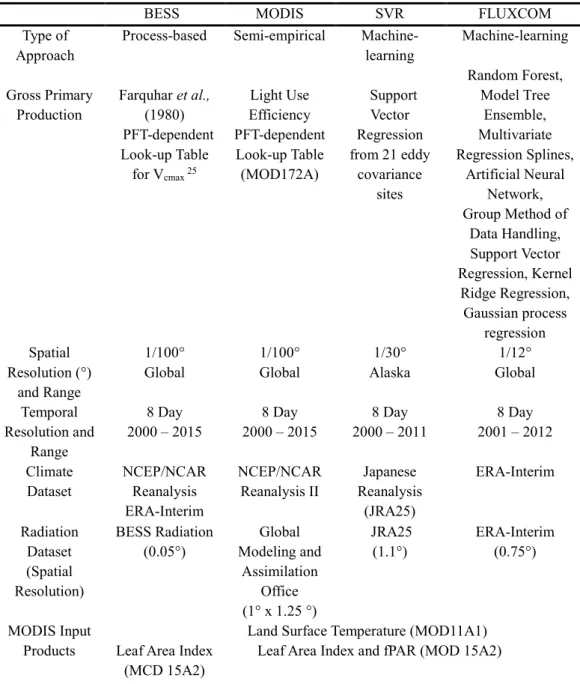
Table 2. Summary of Model Approach and MODIS input forcing data
BESS MODIS SVR FLUXCOM
Type of Approach
Process-based Semi-empirical Machine-learning Machine-learning Gross Primary Production Farquhar et al., (1980) PFT-dependent Look-up Table for Vcmax 25 Light Use Efficiency PFT-dependent Look-up Table (MOD172A) Support Vector Regression from 21 eddy covariance sites Random Forest, Model Tree Ensemble, Multivariate Regression Splines, Artificial Neural Network, Group Method of Data Handling, Support Vector Regression, Kernel Ridge Regression, Gaussian process regression Spatial Resolution (°) and Range 1/100° Global 1/100° Global 1/30° Alaska 1/12° Global Temporal Resolution and Range 8 Day 2000 – 2015 8 Day 2000 – 2015 8 Day 2000 – 2011 8 Day 2001 – 2012 Climate Dataset NCEP/NCAR Reanalysis ERA-Interim NCEP/NCAR Reanalysis II Japanese Reanalysis (JRA25) ERA-Interim Radiation Dataset (Spatial Resolution) BESS Radiation (0.05°) Global Modeling and Assimilation Office (1° x 1.25 °) JRA25 (1.1°) ERA-Interim (0.75°) MODIS Input Products
Land Surface Temperature (MOD11A1) Leaf Area Index
(MCD 15A2)
18 Other MODIS Input Products Aerosol (MOD04_L2) Atmosphere Profile (MOD07_L2) Cloud (MOD06_L2) Albedo (MCD43B3) Surface Temperature (MOD11A1) Surface reflectance - GR (MOD09A2)
NDVI & EVI (MOD13A2) MCD43A2/4 Bidirectional Reflectance Distribution Function Landcover Landcover (MCD12A1) Alaska Geospatial Data Clearinghouse Reference (Ryu et al., 2011,
Jiang and Ryu 2016) (Running et al., 2004, Zhao et al., 2006) (Ueyama et al., 2013) (Tramontana et al., 2016)
2.4 Dataset of climate variables
To examine the relationship of GPP with air temperature, precipitation and shortwave radiation, we used gridded climate data. For air temperature and precipitation, we used monthly CRU (Climate Research Unit) TS2.31 Mean Temperature and CRU T323 Precipitation dataset, respectively, which is monthly gridded data based on daily values with a spatial resolution of 0.5° (Harris et al., 2014). This climate dataset is constructed based upon more than 4500 meteorological stations distributed around the world. This data assembles multiple station variables from numerous data sources into a consistent format. Shortwave radiation data was obtained from the Breathing Earth System Simulator (BESS) at
19
5km, 4 daily spatial temporal resolutions, which was created by merging an atmospheric radiative transfer model with model with an artificial neural network using MODIS atmosphere and land products (Ryu et al., 2018). We used these climate variable data (CRU air temperature, CRU precipitation and BESS shortwave radiation) with latitudes between 71.5°N and 51.5°N and longitudes from -170°W to 140°W in the period during the period between 2001 and 2011. CRU data is available at https://climatedataguide.ucar.edu/climate-data/cru-ts321-gridded-precipitation-and-other-meteorological-variables-1901. BESS shortwave products are publically available at http://environment.snu.ac.kr/ .
2.5 Landcover map
To classify plant functional types (PFTs), we used landcover data from Ueyama
et al., (2013), who regrouped data from Alaska Geospatial Data Clearinghouse to
represent four PFTs: tundra (68 %), evergreen needleleaf forest (26%), deciduous broadleaf forest (4%) and fire scars (0.9%), hereafter called fire (Figure 1). Fire is a new classification in the landcover data which was added as the relationship between CO2 fluxes and environmental and satellite observations on ecosystems
disturbed by fire was substantially different from later successional ecosystems (Randerson et al., 2006, Welp et al., 2007, Ueyama et al., 2013). Fire scars are areas where fire has occurred in the last 10 years based on data from the Alaska Fire
20
Service. 10 years was used as a proxy to determine the appropriate pixel as fire scar based on research showing that approximately 10 years after a fire event, EVI and CO2 uptake during midday was comparable to unburned sites.
2.6 Evaluation and analysis of GPP
To evaluate model performance with the 17 flux tower site data, we extracted the pixel that was closest to the tower using Delaunay Triangulation and nearest neighbor. We used a statistical threshold to remove poor daily flux data and then gap filled using a two-dimensional interpolator to conserve the mean diurnal variation. Subsequently, we averaged daily flux data to 8 days, only selecting days that had less than 25% gap filling. In other words, we discarded 8-day composite data where 6 or more days had been gap filled. For monthly variation we averaged the daily to monthly data, again selecting only monthly data where less than 25% of the data had been gap filled.
To test the performance of models in Alaska, we used linear regression, correlation coefficient (r2), root mean squared error (RMSE), relative RMSE
(rRMSE), bias and relative bias (rBias) between the observed values from flux data and predicted values from BESS, MODIS, SVR and FLUXCOM, using the following equations:
21 𝑅𝑀𝑆𝐸 = √ 1 𝑛∑ (𝑋𝑜𝑏𝑠− 𝑋𝑚𝑜𝑑𝑒𝑙) 2 𝑛 𝑖=1 (Eq. 1)
Relative RMSE (%) = (RMSE / 𝑋̅̅̅̅̅̅ ) x 100 (Eq. 2) 𝑜𝑏𝑠
𝐵𝑖𝑎𝑠 = 𝑋̅̅̅̅̅̅ − 𝑋𝑜𝑏𝑠 ̅̅̅̅̅̅̅̅̅ (Eq. 3) 𝑚𝑜𝑑𝑒𝑙 Relative Bias (%) = (Bias /𝑋̅̅̅̅̅̅ ) x 100 (Eq. 4) 𝑜𝑏𝑠
Where, 𝑋𝑜𝑏𝑠is GPP from flux data, 𝑋𝑚𝑜𝑑𝑒𝑙is GPP estimated by the model and
overbar indicates average.
To investigate the relationship of (IAV) of GPP with climate variables, we aggregated the spatial resolution of BESS (0.01°), MODIS (0.01°), SVR (0.033°) and FLUXCOM (0.083°) to 0.5° grids to compare using the same spatial resolution of climate datasets. The 8 daily composite GPP data were converted to monthly data. We defined growing season as the months when air temperature is above 5°C for each grid cell, assuming that this is when snow has fully melted and leaf has come out so that vegetation may start photosynthesizing (Molau and Molgaard 1996), thus the number of growing season months for each grid cells may be different. We quantified interannual variation and anomaly for just the growing season, as GPP in the winter months is constantly negligible whether winter is relatively warm or
22
cold.
For all analysis, annual growing season anomaly of GPP, air temperature, precipitation and shortwave radiation were used. Anomaly was calculated as the aberration of the ten year mean of the detrended growing season GPP or climate variable. To investigate the response of GPP IAV with climate variables (air temperature, precipitation and shortwave radiation), we used monthly Z Scores, which are growing season anomalies normalized by its standard deviation.
We used Ahlström et al., (2015)’s method to partition the relative contribution of PFTs to interannual variation of GPP in Alaska. For a given flux (GPP), the contribution of IAV of a grid cell or PFT j to the GPP IAV is defined as:
𝑓𝑗 = ∑
𝑥𝑗𝑡 |𝑋𝑡| 𝑋𝑡 𝑡
∑ 𝑋𝑡𝑡 (Eq. 6)
Where 𝑥jt is the flux anomaly for PFT j at time t (in years) and Xt is the global
flux anomaly. Xt is the total flux anomaly, so that 𝑋𝑡 = ∑ 𝑥𝑗 𝑗𝑡. We use this method
to compare the relative contribution of PFTs in driving global GPP IAV, where PFTs with high scores drive the overall variation, while low scores contribute less with the total sum being equal to 1. Further information of this method can be found in
23
the supplementary materials of Ahlström et al., (2015).
To examine which PFT governed the IAV of GPP in Alaska, we partitioned GPP IAV quantifying the relative contribution of each grid cell and then summing up for each PFT. The relative contribution can be negative or positive as it quantifies the relative importance to governing GPP IAV, thus the total sum is 1. Then we examined the magnitude of growing season GPP IAVs during 2001 to 2011, with relative standard deviation. To investigate the spatial and temporal drivers of GPP IAV by PFT, we performed a partial correlation analysis between growing season GPP anomalies and climate variables, air temperature, precipitation and shortwave radiation.
24
3. Results 3.1 Evaluation of Models against flux tower data
Evaluation at the site scale showed that the model performance of BESS, MODIS, SVR and FLUXCOM were substantially different in PFTs.Generally, the four models explained 58% to 82% of the variability in GPP over the different plant functional types (Figure 2 and Table 3). Among the 4 different PFTs all models, whether process based or machine learning, performed better in ENF and DBF with high r2, low RMSE and small bias, compared to tundra and recently disturbed sites
by fire that had relatively low r2, high RMSE and large bias.
Table 3. Evaluation of BESS, MODS, SVR and FLUXCOM in Alaska using r2, RMSE, relative
25 bias are gC m-2 d-1.
In general, rRMSE was smaller in ENF and DBF compared to tundra and fire sites for all models, showing that model performance is still relatively weaker in tundra and fire sites. BESS and MODIS overestimated in tundra regions and underestimated in the boreal forest, whereas, SVR and FLUXCOM tended to underestimate GPP in tundra regions compared to boreal forest. In ENF, models
PFT Sites
BESS GPP MODIS GPP SVR GPP FLUXCOM GPP
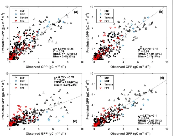
r² RMSE (rRMSE) Bias (rBias) r² RMSE (rRMSE) Bias (rBias) r² RMSE (rRMSE) Bias (rBias) r² RMSE (rRMSE) Bias (rBias) ENF 6 0.82 1.01 (55%) 0.08 (4%) 0.81 1.06 (57%) -0.06 (-3.2%) 0.75 1.29 (70%) -0.55 (-30%) 0.88 0.77 (41%) -0.01 (-5%) DBF 1 0.93 0.68 (41%) 0.35 (21%) 0.95 0.57 (38%) 0.08 (5%) 0.54 1.9 (125%) -0.85 (-56%) 0.96 0.86 (54%) -0.42 (-28%) Tundra 7 0.69 1.25 (184%) 0.67 (99%) 0.66 0.90 (151%) 0.24 (40%) 0.66 0.50 (85%) -0.07 (-11%) 0.65 0.50 (85%) -0.05 (-8%) Fire 3 0.65 1.04 (95%) 0.51 (46%) 0.65 1.10 (106%) 0.39 (38%) 0.31 1.01 (98%) -0.24 (23%) 0.68 0.66 (63%) 0.09 (8.7%) Overall 17 0.74 1.12 (90%) 0.41 (33%) 0.75 1.01 (81%) 0.17 (14%) 0.65 1.07 (86%) -0.27 (-22%) 0.85 0.69 (54%) -0.07 (-6%)
26
captured 75% to 88% of the variability in GPP, where rRMSE ranged from 41% to 70%. SVR, FLUXCOM and MODIS had negative rBiases in ENF, -30%, -5% and -3.2%, respectively, while BESS had a positive rBias of 4%. For DBF, models performed best in capturing over 90% of the variability in GPP, except for SVR, which also had the largest rRMSE (125%). Both BESS and MODIS showed a positive rBias (21% and 5%, respectively) while SVR and FLUXCOM exhibited a negative rBias (-56% and -28%, respectively) in DBF. In Tundra and Fire, the low productive sites, GPP was overestimated by the process-based and semi-empirical model, in contrast to the highly productive sites, ENF and DBF, whereas the machine-learning models underestimated GPP in all sites except fire, as illustrated in Figure 2. The data driven statistical models, clearly underestimated GPP with high relative biases in both ENF and DBF (SVR rBias = -56%, rRMSE = 70%; FLUXCOM rBias = -28%, rRMSE = 41%) but had a smaller relative bias in tundra and fire sites (SVR rBias = -11%, rRMSE = 85%; FLUXCOM rBias = -8%, rRMSE = 85%).
27
Figure 2 Evaluation of modeled GPP at a monthly time scale. (a) BESS, (b) MODIS, (c) SVR and (d) FLUXCOM with eddy covariance flux data. GPP from ENF and DBF sites are nearly twice of tundra GPP. GPP in fire and tundra sites are relatively much lower
3.2 IAV of GPP
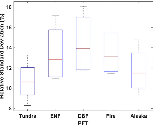
We found that the boreal forest in Alaska had the largest magnitude of GPP IAV. DBF showed the largest magnitude of growing season GPP IAVs with the largest relative standard deviation of 13.9 ± 0.03%. The magnitude of GPP IAV in ENF is 13.4 ± 0.3% with the interior of Alaska exhibiting a greater variation compared to
28
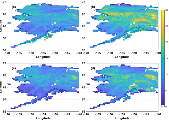
the lower coastal regions of ENF. Fire showed a similar variability as ENF with a relative standard deviation of 12.8 ± 0.02%. Tundra had the lowest relative standard deviation of 10.6 ± 0.02%, with the Seward Peninsula and the north western part of North Slope exhibiting a higher magnitude in the variability of GPP. In contrast, the southern tundra regions and the other part of the northernmost region of Alaska showed the lowest degree of variability in GPP IAV (Figure 3). DBF is a highly productive area that has the most variation in the magnitude of GPP in the growing season. Furthermore, MODIS showed the highest degree of variation in all PFTs, followed by FLUXCOM, BESS and SVR which is a consequence of different approaches for each model leading to such variations (Figure 4). The boreal forest had the largest magnitude in the IAV of GPP with part of tundra regions also showing a high degree of variation, suggesting that vegetation production in these regions may contribute substantially to GPP IAV in Alaska.
29
Figure 3 The Relative standard deviation (%) of GPP IAV (a) BESS, (b) MODIS, (c) SVR and (d) FLUXCOM.
30
Figure 4 Averaged relative standard deviation of GPP IAV.
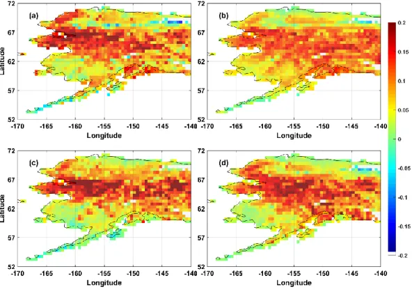
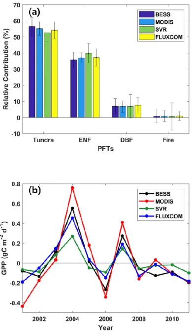
The pattern of growing season GPP IAV was similar across the different PFTs with varying magnitudes (Figure 6), except for fire areas in SVR. Tundra had the highest relative contribution to the interannual variation of GPP with the largest fraction of 55%, exceeding ENF (38%), DBF (7%) and fire (0.8%) in Alaska (Figure 6a). All of the models, BESS, MODIS, SVR and FLUXCOM, displayed a similar spatial and temporal pattern in the IAV of growing season GPP. The spatial pattern of the relative contribution of each pixel to growing season GPP IAV varied
31
across the region of Alaska. The growing season GPP mean is relatively small in tundra compared to the other PFTs, but tundra in the Seward Peninsula and western part of the North Slope contributed up to 0.2% of the IAV of GPP growing season, which is similar to the relative contribution of pixels in DBF to GPP IAV. Overall, the sum of relative pixel contribution for each PFTs show that tundra contributed the most to the IAV of GPP as it covered up to 68% of Alaska (Figure 6b). Despite the magnitude of the flux in PFTs, the percent of land cover fraction for each respective PFT cover resulted in contributing most to the IAV of GPP. 0.06 %, 0.03%, 0.05% and 0.03% of the pixels had negative relative contribution to GPP IAV for BESS, MODIS, SVR and FLUXCOM, respectively. The negative relative contributions were generally located in the north eastern alpine regions of Alaskan. BESS and SVR showed more negative relative contribution in the southern tail of Alaska.
32
Figure 5 Relative contribution (%) of each grid cell to GPP IAV. (a) BESS, (b) MODIS. (c) SVR and (d) FLUXCOM.
33
Figure 6 (a) The sum of relative contribution of GPP IAV each PFT, and the (b) the IAV of GPP from 2001 to 2011 in Alaska.
34
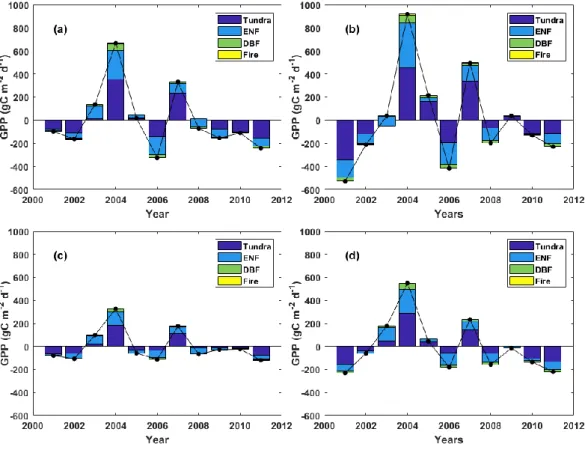
The year to year relative contribution of PFT to GPP IAV varies where Tundra was the major contributor followed by ENF, DBF and Fire (Figure 7). All models show that Tundra was the major contributor to GPP IAV in 2001, 2002, 2004, 2005, 2006, 2008, 2009, 2010, 2011, 2012, whereas ENF contributed most to GPP IAV in 2003 and 2008 when GPP anomaly was close to the mean. DBF and Fire contributed to the IAV of GPP every year in relatively smaller quantity due to its smaller area. In the warmer years the relative contribution of PFT to GPP IAV was positive while in the colder years the relative contribution of PFT to GPP IAV was negative.
35
Figure 7 Relative contribution of PFT to GPP. (a) BESS, (b) MODIS. (c) SVR and (d) FLUXCOM. The black line indicates GPP anomaly for each year over Alaska
3.3 Relationship between IAV of GPP and Climate Variables
Air temperature was the most dominant driver of the spatial and temporal pattern of GPP IAV for all PFTs. As illustrated in Figure 8, the spatial pattern between air temperature and GPP was similar, where 81%, 87%, 78%, 82% of the
36
pixels had a significant (p Value < 0.1) partial correlation for BESS, MODIS, SVR and FLUXCOM, respectively, of which more than 50% of the pixels were located in tundra, 20 % in ENF, 0.04 % in DBF and 0.005 % in the fire regions. Across all PFTs, air temperature had the highest positive correlation followed by radiation, indicating that the high latitude ecosystems are co-limited by both air temperature and shortwave radiation (Figure 8). In Alaska, it is interesting to note that GPP in the northern tip of Alaska is not driven by air temperature but solar radiation (Figure 8). In contrast, there are much fewer areas that are affected by precipitation, with only about 16 – 18% of the pixels showing a significant (p Value < 0.1) partial correlation coefficient. There is a decrease of GPP when there is precipitation in the northern most part of tundra and the southern part of coastal tundra, which emphasize that tundra GPP does not depend on snowfall and rain for water as these regions are underlain by permafrost.
37 Figure 8 RGB composite of climatic drivers
As illustrated in Figure 5, the Seward Peninsula and the western North Slope contributed up to 0.2% of GPP IAV, which is similar to the pixels in the boreal forest that is found in the Interior of Alaska. In contrast, the contribution of the Arctic Coastal Plain and North Slope of Alaska and southern tundra in Alaska to GPP was smaller than 0.1%. The spatial pattern of relative contribution to GPP IAV is remarkably similar to the areas where both air temperature and radiation drive GPP (Figure 8). The Arctic Coastal Plain and southern tundra regions, which has a
38
partial correlation coefficient with air temperature contributed less to GPP IAV than the areas where both air temperature and radiation have a relationship with GPP. West of the Brooks Range, the alpine regions, and Alaska Peninsula show a small negative contribution to air temperature corresponding to the positive correlations with precipitation. The relative contribution of pixels to GPP in BESS, MODIS, SVR and FLUXCOM was associated with both air temperature and radiation, displaying a similar pattern although they had different spatial pattern and magnitude (Figure 9). The negative relative contribution is from tundra when the driving factors are both radiation and precipitation. Air temperature and radiation were co-dominantly associated to the GPP IAV for all PFTs in Alaska. At one point in the growing season, daylight hours may be up to 24 hours, which may enhance vegetation productivity (Bliss et al., 1973). Across the PFTs for Alaska air temperature and radiation were the most important climate factors that influence GPP year to year variability.
39
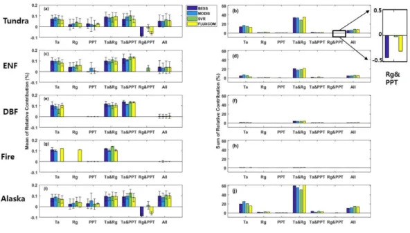
Figure 9 The mean and sum of relative contribution to GPP IAV for PFT. Mean of relative contribution for a) Tundra c) ENF e) DBF g) Fire and i) Alaska and the sum of relative contribution in b) Tundra d) ENF f) DBF h) Fire and j) Alaska when there is a partial correlation with Ta (air temperature), Rg (radiation), PPT (precipitation), Ta & Rg (air temperature and radiation), Ta & PPT (air temperature and precipitation), Rg & PPT (radiation and precipitation) and All (air temperature, precipitation and radiation). The error bar shows the variation of relative contribution for each case.
The average partial correlation coefficient for the whole of Alaska shows that growing season GPP was positively correlated to growing season temperature (r = 0.8) and radiation (r = 0.7) but a small negative correlation with precipitation (r = -0.2). Except for MODIS, the other models show that only DBF has a positive correlation coefficient with precipitation. In the fire region, BESS, SVR and FLUXCOM GPP were not associated with precipitation, implying that these
40
ecosystems recover from fire disturbance regardless of precipitation. There is high variation in precipitation correlation coefficient with GPP. The relationships between growing season GPP and climate variables vary greatly among PFTs but these results highlight that both air temperature and shortwave radiation are the limiting factor that act together upon GPP to control its year to year variation.
41
4. Discussion 4.1 Model Performance across different PFTs
The performance of BESS, MODIS, SVR and FLUXCOM at a site scale across PFTs differed substantially, where all models showed a better performance in the boreal forest compared to tundra and fire sites (Table 3). BESS, MODIS, SVR and FLUXCOM could capture 65% to 85% of the seasonal variability in GPP but they had a larger uncertainty in tundra compared to boreal forest. Fisher et al., (2014) reported that GPP had the second highest uncertainty (225%) among the different carbon flux components after soil carbon from terrestrial biosphere models, where tundra exhibited more uncertainty compared to boreal forest (Ueyama et al., 2013, Tramontana et al., 2016). One precaution to take in model evaluation is that the eddy covariance flux towers could not represent all the ecosystems in Alaska, which has a highly heterogeneous landscape and topography (Williams et al., 2006, Shaver et al., 2007). Our model evaluation did not include eddy covariance flux towers situated in white spruce and birch forests, various aged ecosystems after fire, wetlands, bogs and other types of shrubland (Flemming 1997, Walker et al., 2005). There was one DBF site (white spruce forest) and tundra sites were only located in the northern region of Alaska (Figure 1), thus excluding tundra ecosystems composed of tall or low shrubs, alpine or moist herbaceous tundra.
42
GPP, whereas the process-based and semi-empirical models tended to overestimate GPP in Alaska. SVR and FLUXCOM are limited by data, which were from only a few types of arctic ecosystems with most of the data available in the growing season (Kwon et al., 2006, Ueyama et al., 2013). FLUXCOM used 224 flux tower sites from FLUXNET La Thulie synthesis dataset of which 6 sites were located in Alaska. There are 3 sites found in the Alaskan Arctic tundra regions (Atqasuk, Barrow and Ivotuk) and the other 3 in the Alaska boreal forest regions (Bonzona Creek 1, Bonzona Creek 2 and Bonzona Creek 3). In contrast, SVR upscaled from 21 flux tower sites to a regional scale in Alaska, but showed the least spatial and temporal variation of GPP. Moreover, GPP data is an indirect measurement of the eddy covariance system, thus it is subject to uncertainties in the flux partitioning methods. Turner et al., (2006) traced the overestimation of MODIS GPP in tundra biomes to unrealistically high values of fPAR (fraction of absorbed photosynthetically active radiation) and underestimation of GPP in highly productive sites (i.e. DBF and ENF) due to low values of vegetation LUE (Light Use Efficiency). There have been significant improvements and updates of MODIS fPAR, including the removal of cloud contamination, but studies still show that estimation of GPP with MODIS fPAR and maximum LUE from the biome look-up-table has uncertainty in capturing seasonal and yearly variation (Sjöström et al., 2013, Cheng et al., 2014, Wang et al., 2017). Cheng et al., (2014) demonstrated that GPP estimated using
43
fPAR, from chlorophyll in leaves, and site-specific maximum LUE resulted in a higher accuracy than GPP derived from MODIS fPAR and maximum LUE from the biome look-up-table. Recently, an evaluation of the latest MOD17A2H GPP that is derived from the most updated MODIS products, still traced the sources of error to MODIS fPAR (MOD15A2H Collection 6), LUE and landcover misclassification (Wang et al., 2017). Not only BESS and MODIS used MODIS fPAR products but also SVR and FLUXCOM, which may have led to such high uncertainty in tundra. The key photosynthesis parameter in BESS is Vcmax (maximum carboxylation rate)
and LAI, which may have also led to bias and error in the estimation of GPP. The high error and bias in BESS may be due to the largely unavailable Vcmax data in the
Arctic (Rogers 2014), where other terrestrial biosphere models are also still found to underestimate the photosynthetic capacity and CO2 assimilation due to this
parameter (Walker et al., 2014, Rogers et al., 2017). Hence tundra still remains a challenging PFT for both process-based and machine-learning approaches.
4.2 IAV of GPP
The IAV of GPP had a similar pattern with the IAV of air temperature and radiation, where all models showed a consistent spatial and temporal pattern of GPP IAV from 2001 to 2011 (Figure 3 and Figure 10). Other studies have also reported a similar IAV of GPP in Alaska (Ueyama et al., 2013, Mekonnen et al., 2016).
44
Mekonnen et al., (2016) reported the GPP IAV in North America was related with the cold phase of El Niño Southern Oscillation (ENSO) and negative Multivariate ENSO Index that has led to major droughts in 2001, 2002, 2008 and 2009, leading to small GPP anomalies. The results also show that that there were small or negative GPP anomalies during 2001, 2002, 2008 and 2009 (Figure 11). In contrast, during the warmer years GPP anomalies were positive, especially during 2004 and 2007 which were recorded as particularly warm and dry years with many fire events.
Overall, the boreal forest exhibited a larger variability of GPP than in tundra, which may be explained by the complexity of the canopy structure (Figure 3) (Zhou
et al., 2017). The complexity of canopy structure increases with a non-linear change
in biomass, cover and height of the understory and overstory, as we transition from tundra to shrub tundra to closed canopy forest (Thompson et al., 2004, Beringer et al., 2005). In particular, the understory variation increases significantly along the gradient from tundra to forest. A previous study shows that in a sparsely populated ENF, the seasonal variation of the understory vegetation contributed significantly to the IAV of GPP as it was more responsive to the environmental controlling factors (Ueyama et al., 2006). Therefore, the higher variability of GPP in the boreal forest could be explained by the larger biomass of the forest and the high variability of the understory canopy. Furthermore, the various stand age of the forest contributes to
45
the larger variation of GPP in the boreal forest (Goulden et al., 2006). Our results show that tundra contributed most to the IAV of GPP with up to 55%, which is expected as it was the largest PFT covering 68% of Alaska. The relative contribution of tundra to GPP IAV is relatively less because of the negative contribution of tundra in the north eastern Brooks Range and Alaska Peninsular to GPP IAV (Figure 3). In contrast, ENF contribution (38%) is relatively higher to GPP IAV than its area (26%) as their average relative contribution was higher than tundra with no negative contribution.
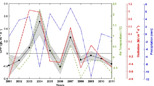
Figure 10 The IAV pattern of GPP (black solid line) in Alaska from 2001 to 2011 with air temperature (green dashed line), precipitation (red dotted line) and radiation (blue dotted and dashed line). The black solid line represents the ensemble of BESS, MODIS, SVR and FLUXCOM while the shaded area in grey represents the variation of the models.
46
We found that GPP IAV in Alaska was driven by both air temperature and radiation across all PFTs (Figure 8 and Figure11). This is in agreement with other research showing that the northern vegetation is most sensitive to air temperature and radiation (Nemani et al., 2003, Mekonnen et al., 2016, Seddon et al., 2016, Liang et al., 2017). Light use efficiency increases with temperature, only in cold regions. This may explain why GPP IAV was co-limited by air temperature and radiation across PFTs where the efficiency of vegetation transforming absorbed radiation into plant biomass is enhanced with increasing temperature (Schwalm et al., 2006, Garbulsky et al., 2010). Ueyama et al., (2006) also reported that light use efficiency was limited by low temperatures in a black spruce forest. In Alaska, when air temperature increases vegetation productivity could be enhanced by efficiently absorbing radiation compared to colder years.
47
5. Conclusion
In this study we examined the spatial and temporal IAV of GPP across Alaska from 2001 to 2011 using four satellite based GPP products. Model performance differed substantially among PFTs, showing a better performance in the boreal forest compared to tundra. GPP in tundra had the largest relative contributed to the IAV of GPP as it has the largest area among PFTs. In particular, GPP from tundra in the Seward Peninsula and the western Brooks Range highly contributed to IAV of GPP along with the interior of Alaska. The spatial and temporal variation of GPP IAV was relatively higher in the boreal forest than tundra. The relationships between GPP and climate variables vary among PFTs depending on the region due to topography, but both air temperature and radiation were the major climate variables that governed GPP to control its year to year variation. This study highlights that vegetation response is sensitive to air temperature and radiation IAV, which controls the year to year spatial and temporal variability of GPP. Therefore, in the high latitudes, warming or cooling as a result of climate change could significantly impact the magnitude and trajectory of the IAV of land-atmosphere interaction of carbon dioxide.
48
References
Ahlström, A., M. R. Raupach, Guy Schurgers, Benjamin Smith, Almut Arneth, Martin Jung, Markus Reichstein, JosepG. Canadell, Pierre Friedlingstein, Atul K. Jain, Etsushi Kato, Benjamin Poulter, Stephen Sitch, Benjamin D. Stocker, Nicolas Viovy, Ying Ping Wang, Andy Wiltshire, Sönke Zaehle and N. Zeng1 (2015). "The dominant role of semi-arid ecosystems in the trend and variability of land CO2 sink." Science 348(637): 895-899.
Beck, P. S. A. and S. J. Goetz (2012). "Corrigendum: Satellite observations of high northern latitude vegetation productivity changes between 1982 and 2008: ecological variability and regional differences." Environmental Research Letters 7(2): 029501. DOI: 10.1088/1748-9326/7/2/029501
Bekryaev, R. V., I. V. Polyakov and V. A. Alexeev (2010). "Role of Polar Amplification in Long-Term Surface Air Temperature Variations and Modern Arctic Warming." Journal of Climate 23(14): 3888-3906. DOI: 10.1175/2010jcli3297.1
Beringer, J., F. S. Chapin, C. C. Thompson and A. D. McGuire (2005). "Surface energy exchanges along a tundra-forest transition and feedbacks to climate." Agricultural and Forest Meteorology 131(3-4): 143-161. DOI: 10.1016/j.agrformet.2005.05.006
Bieniek, P. A. and J. E. Walsh (2017). "Atmospheric circulation patterns associated with monthly and daily temperature and precipitation extremes in Alaska." International Journal of Climatology. DOI: 10.1002/joc.4994
Black, T. A., W. J. Chen, A. G. Barr, M. A. Arain, Z. Chen, Z. Nesic, E. H. Hogg, H. H. Neumann and P. C. Yang (2000). "Increased carbon sequestration by a boreal deciduous forest in years with a warm spring." Geophysical Research Letters 27(9): 1271-1274. DOI: 10.1029/1999gl011234
Bliss, L. C., G. M. Courtin, D. L. Pattie, R. R. Riewe, D. W. A. Whitfield and P. Widden (1973). "Arctic and tundra ecosystems." Annu. Rev. Ecol. Syst 4: 359-399.
ChapinIII, F. S., M. Sturm, M. C. Serreze, J. P. McFadden, J. R. Key, A. H. Lloyd, A. D. McGuire, T. S. Rupp, A. H. Lynch, J. P. Schimel, J. Beringer, W. L. Chapman, H. E. Epstein, E. S. Euskirchen, L. D. Hinzman, G. Jia, C.-L. Ping, K. D. Tape, C. D. C. Thompson, D. A. Walker and J. M. Welker (2005). "Role of Land-Surface Changes in Arctic Summer Warming." Science 310(5748): 657 - 660.
Cheng, Y.-B., Q. Zhang, A. I. Lyapustin, Y. Wang and E. M. Middleton (2014). "Impacts of light use efficiency and fPAR parameterization on gross primary production modeling." Agricultural and Forest Meteorology 189-190: 187-197. DOI: 10.1016/j.agrformet.2014.01.006
Commane, R., J. Lindaas, J. Benmergui, K. A. Luus, R. Y. Chang, B. C. Daube, E. S. Euskirchen, J. M. Henderson, A. Karion, J. B. Miller, S. M. Miller, N. C. Parazoo, J. T. Randerson, C. Sweeney, P.
49
Tans, K. Thoning, S. Veraverbeke, C. E. Miller and S. C. Wofsy (2017). "Carbon dioxide sources from Alaska driven by increasing early winter respiration from Arctic tundra." Proc Natl Acad Sci U S A. DOI: 10.1073/pnas.1618567114
Cramer, W., D.W.Kicklighter, A.Bondeau, B. M. III, G. Churkina, B.Nemry, A.Ruimy and A.L.Schloss (1999). "Comparing Global Models of Terrestrial Net Primary Productivity: overview and key results." Glob Chang Biol 5: 1 - 15.
Euskirchen, E. S., M. S. Bret-Harte, G. J. Scott, C. Edgar and G. R. Shaver (2012). "Seasonal patterns of carbon dioxide and water fluxes in three representative tundra ecosystems in northern Alaska." Ecosphere 3(1): art4. DOI: 10.1890/es11-00202.1
Euskirchen, E. S., M. S. Bret-Harte, G. R. Shaver, C. W. Edgar and V. E. Romanovsky (2016). "Long-Term Release of Carbon Dioxide from Arctic Tundra Ecosystems in Alaska." Ecosystems. DOI: 10.1007/s10021-016-0085-9
Farquhar, G. D., S. v. Caemmerer and J. A. Berry (1980). "A biochemical model of photosynthetic CO2 assimilation in leaves of C3 species." Planta 149: 78 - 90.
Fisher, J. B., M. Sikka, W. C. Oechel, D. N. Huntzinger, J. R. Melton, C. D. Koven, A. Ahlström, M. A. Arain, I. Baker, J. M. Chen, P. Ciais, C. Davidson, M. Dietze, B. El-Masri, D. Hayes, C. Huntingford, A. K. Jain, P. E. Levy, M. R. Lomas, B. Poulter, D. Price, A. K. Sahoo, K. Schaefer, H. Tian, E. Tomelleri, H. Verbeeck, N. Viovy, R. Wania, N. Zeng and C. E. Miller (2014). "Carbon cycle uncertainty in the Alaskan Arctic." Biogeosciences 11(15): 4271-4288. DOI: 10.5194/bg-11-4271-2014
Flemming, M. (1997). "A statewide vegetation map of Alaska using phenological classificaiton of AVHRR data. In: Proceedings of the Second Circumpolar Arctic Vegetation Mapping Workshop, Arendal, Norway." 25-26.
Garbulsky, M. F., J. Peñuelas, D. Papale, J. Ardö, M. L. Goulden, G. Kiely, A. D. Richardson, E. Rotenberg, E. M. Veenendaal and I. Filella (2010). "Patterns and controls of the variability of radiation use efficiency and primary productivity across terrestrial ecosystems." Global Ecology and Biogeography 19(2): 253-267. DOI: 10.1111/j.1466-8238.2009.00504.x
Goulden, M. L., G. C. Winston, A. M. S. McMillan, M. E. Litvak, E. L. Read, A. V. Rocha and J. Rob Elliot (2006). "An eddy covariance mesonet to measure the effect of forest age on land-atmosphere exchange." Global Change Biology 12(11): 2146-2162. DOI: 10.1111/j.1365-2486.2006.01251.x
Goulden, M. L., S. Wofsy, J. W. Harden, S. E. Trumbore, P. M. Crill, S. T. Gower, T. Fries, B. C. Daube, S. M. Fan, D. J. Sutton, A. Bazzaz and J. W. Munger (1998). "Sensitivity of Boreal Forest C
50 balance to soil thaw." Science 279: 214-217.
Guay, K. C., P. S. Beck, L. T. Berner, S. J. Goetz, A. Baccini and W. Buermann (2014). "Vegetation productivity patterns at high northern latitudes: a multi-sensor satellite data assessment." Glob Chang Biol 20(10): 3147-3158. DOI: 10.1111/gcb.12647
Harazono, Y., M. Mano, A. Miyata and R. C. Zulueta (2003). "Interannual carbon dioxide uptake of a wet sedge tundra ecosystem in the Arctic." Tellus 55B: 215-231.
Harris, I., P. D. Jones, T. J. Osborn and D. H. Lister (2014). "Updated high-resolution grids of monthly climatic observations - the CRU TS3.10 Dataset." International Journal of Climatology 34(3): 623-642. DOI: 10.1002/joc.3711
Huntzinger, D. N., C. Schwalm, A. M. Michalak, K. Schaefer, A. W. King, Y. Wei, A. Jacobson, S. Liu, R. B. Cook, W. M. Post, G. Berthier, D. Hayes, M. Huang, A. Ito, H. Lei, C. Lu, J. Mao, C. H. Peng, S. Peng, B. Poulter, D. Riccuito, X. Shi, H. Tian, W. Wang, N. Zeng, F. Zhao and Q. Zhu (2013). "The North American Carbon Program Multi-Scale Synthesis and Terrestrial Model Intercomparison Project – Part 1: Overview and experimental design." Geoscientific Model Development 6(6): 2121-2133. DOI: 10.5194/gmd-6-2121-2013
Ito, A., M. Inatomi, D. N. Huntzinger, C. Schwalm, A. M. Michalak, R. Cook, A. W. King, J. Mao, Y. Wei, W. M. Post, W. Wang, M. A. Arain, S. Huang, D. J. Hayes, D. M. Ricciuto, X. Shi, M. Huang, H. Lei, H. Tian, C. Lu, J. Yang, B. Tao, A. Jain, B. Poulter, S. Peng, P. Ciais, J. B. Fisher, N. Parazoo, K. Schaefer, C. Peng, N. Zeng and F. Zhao (2016). "Decadal trends in the seasonal-cycle amplitude of terrestrial CO2 exchange resulting from the ensemble of terrestrial biosphere models." Tellus B: Chemical and Physical Meteorology 68(1): 28968. DOI: 10.3402/tellusb.v68.28968
Iwata, H., Y. Harazono and M. Ueyama (2012). "The role of permafrost in water exchange of a black spruce forest in Interior Alaska." Agricultural and Forest Meteorology 161: 107-115. DOI: 10.1016/j.agrformet.2012.03.017
Iwata, H., M. Ueyama, Y. Harazono, S. Tsuyuzaki, M. Kondo and M. Uchida (2011). "Quick Recovery of Carbon Dioxide Exchanges in a Burned Black Spruce Forest in Interior Alaska." Sola 7: 105-108. DOI: 10.2151/sola.2011-027
Jeong, S.-J., C.-H. Ho, H.-J. Gim and M. E. Brown (2011). "Phenology shifts at start vs. end of growing season in temperate vegetation over the Northern Hemisphere for the period 1982-2008." Global Change Biology 17(7): 2385-2399. DOI: 10.1111/j.1365-2486.2011.02397.x
Jiang, C. and Y. Ryu (2016). "Multi-scale evaluation of global gross primary productivity and evapotranspiration products derived from Breathing Earth System Simulator (BESS)." Remote Sensing of Environment 186: 528-547. DOI: 10.1016/j.rse.2016.08.030
51
Kwon, H.-J., W. C. Oechel, R. C. Zulueta and S. J. Hastings (2006). "Effects of climate variability on carbon sequestration among adjacent wet sedge tundra and moist tussock tundra ecosystems." Journal of Geophysical Research 111(G3). DOI: 10.1029/2005jg000036
Liang, W., Y. Lu, W. Zhang, S. Li, Z. Jin, P. Ciais, B. Fu, S. Wang, J. Yan, J. Li and H. Su (2017). "Grassland gross carbon dioxide uptake based on an improved model tree ensemble approach considering human interventions: global estimation and covariation with climate." Glob Chang Biol 23(7): 2720-2742. DOI: 10.1111/gcb.13592
McGuire, A. D., F. S. Chapin, J. E. Walsh and C. Wirth (2006). "Integrated Regional Changes in Arctic Climate Feedbacks: Implications for the Global Climate System*." Annual Review of Environment and Resources 31(1): 61-91. DOI: 10.1146/annurev.energy.31.020105.100253
Mekonnen, Z. A., R. F. Grant and C. Schwalm (2016). "Contrasting changes in gross primary productivity of different regions of North America as affected by warming in recent decades." Agricultural and Forest Meteorology 218-219: 50-64. DOI: 10.1016/j.agrformet.2015.11.016
Molau, U. and P. Molgaard (1996). "International Tundra Experiment Mannual." Danish Polar Center, Copenhagen, Denmark.
Nakai, T., Y. Kim, R. C. Busey, R. Suzuki, S. Nagai, H. Kobayashi, H. Park, K. Sugiura and A. Ito (2013). "Characteristics of evapotranspiration from a permafrost black spruce forest in interior Alaska." Polar Science 7(2): 136-148. DOI: 10.1016/j.polar.2013.03.003
Nauta, A. L., M. M. P. D. Heijmans, D. Blok, J. Limpens, B. Elberling, A. Gallagher, B. Li, R. E. Petrov, T. C. Maximov, J. van Huissteden and F. Berendse (2014). "Permafrost collapse after shrub removal shifts tundra ecosystem to a methane source." Nature Climate Change 5(1): 67-70. DOI: 10.1038/nclimate2446
Nemani, R. R., C. D. Keeling, H. Hashimoto, W. M. Jolly, S. C. Piper, C. J. Tucker, R. B. Myneni and S. W. Running (2003). "Climate-driven increases in global terrestrial net primary production from 1982 to 1999." Science 300(5625): 1560-1563. DOI: 10.1126/science.1082750
Oechel, W. C., S. J. Hastings, G. Vourlitis, M. Jenkins, G. Riecher and N. Grulke (1993). "Recent changes of the arctic tundra ecosystem from a net carbon dioxide sink to source." Nature Lett. 361: 520 - 523.
Park, H., S.-J. Jeong, C.-H. Ho, J. Kim, M. E. Brown and M. E. Schaepman (2015). "Nonlinear response of vegetation green-up to local temperature variations in temperate and boreal forests in the Northern Hemisphere." Remote Sensing of Environment 165: 100-108. DOI: 10.1016/j.rse.2015.04.030
52
Park, T., S. Ganguly, H. Tømmervik, E. S. Euskirchen, K.-A. Høgda, S. R. Karlsen, V. Brovkin, R. R. Nemani and R. B. Myneni (2016). "Changes in growing season duration and productivity of northern vegetation inferred from long-term remote sensing data." Environmental Research Letters 11(8): 084001. DOI: 10.1088/1748-9326/11/8/084001
Piao, S., P. Ciais, P. Friedlingstein, P. Peylin, M. Reichstein, S. Luyssaert, H. Margolis, J. Fang, A. Barr, A. Chen, A. Grelle, D. Y. Hollinger, T. Laurila, A. Lindroth, A. D. Richardson and T. Vesala (2008). "Net carbon dioxide losses of northern ecosystems in response to autumn warming." Nature 451(7174): 49-52. DOI: 10.1038/nature06444
Piao, S., Z. Liu, T. Wang, S. Peng, P. Ciais, M. Huang, A. Ahlstrom, J. F. Burkhart, F. Chevallier, I. A. Janssens, S.-J. Jeong, X. Lin, J. Mao, J. Miller, A. Mohammat, R. B. Myneni, J. Peñuelas, X. Shi, A. Stohl, Y. Yao, Z. Zhu and P. P. Tans (2017). "Weakening temperature control on the interannual variations of spring carbon uptake across northern lands." Nature Climate Change 7(5): 359-363. DOI: 10.1038/nclimate3277
Piao, S., H. Nan, C. Huntingford, P. Ciais, P. Friedlingstein, S. Sitch, S. Peng, A. Ahlstrom, J. G. Canadell, N. Cong, S. Levis, P. E. Levy, L. Liu, M. R. Lomas, J. Mao, R. B. Myneni, P. Peylin, B. Poulter, X. Shi, G. Yin, N. Viovy, T. Wang, X. Wang, S. Zaehle, N. Zeng, Z. Zeng and A. Chen (2014). "Evidence for a weakening relationship between interannual temperature variability and northern vegetation activity." Nat Commun 5: 5018. DOI: 10.1038/ncomms6018
Piao, S., S. Sitch, P. Ciais, P. Friedlingstein, P. Peylin, X. Wang, A. Ahlstrom, A. Anav, J. G. Canadell, N. Cong, C. Huntingford, M. Jung, S. Levis, P. E. Levy, J. Li, X. Lin, M. R. Lomas, M. Lu, Y. Luo, Y. Ma, R. B. Myneni, B. Poulter, Z. Sun, T. Wang, N. Viovy, S. Zaehle and N. Zeng (2013). "Evaluation of terrestrial carbon cycle models for their response to climate variability and to CO2
trends." Glob Chang Biol 19(7): 2117-2132. DOI: 10.1111/gcb.12187
Ping, C.-L., G. J. Michaelson, M. T. Jorgenson, J. M. Kimble, H. Epstein, V. E. Romanovsky and D. A. Walker (2008). "High stocks of soil organic carbon in the North American Arctic region." Nature Geosci 1(9): 615-619. DOI: http://www.nature.com/ngeo/journal/v1/n9/suppinfo/ngeo284_S1.html
Randerson, J. T., H. Liu, M. G. Flanner, S. D. Chambers, Y. Jin, P. G. Hess, G. Pfister, M. C. Mack, K. K. Treseder, L. R. Welp, F. S. Chapin, J. W. Harden, M. L. Goulden, E. Lyons, J. C. Neff, E. A. G. Schuur and C. S. Zender (2006). "Impact of boreal forest fire on climate warming." Science 314: 1130 - 1132.
Rocha, A. V. and G. R. Shaver (2011). "Burn severity influences postfire CO2 exchange in arctic
tundra." Ecological Applications 21(2): 477-489.
Rogers, A. (2014). "The use and misuse of V(c,max) in Earth System Models." Photosynth Res 119(1-2): 15-29. DOI: 10.1007/s11120-013-9818-1