1
Time-Dependent Optimal Heater Control Using Finite Difference Method
Li Zhen-Zhe
†
, Heo Kwang-Su*, Choi Jun-Hoo* and Seol Seoung-Yun**
Key Words : Thermoforming, Finite Difference Method, Optimization Abstract
Thermoforming is one of the most versatile and economical process to produce polymer products. The drawback of thermoforming is difficult to control thickness of final products. Temperature distribution affects the thickness distribution of final products, but temperature difference between surface and center of sheet is difficult to decrease because of low thermal conductivity of ABS material. In order to decrease temperature difference between surface and center, heating profile must be expressed as exponential function form. In this study, Finite Difference Method was used to find out the coefficients of optimal heating profiles. Through investigation, the optimal results using Finite Difference Method show that temperature difference between surface and center of sheet can be remarkably minimized with satisfying Temperature of Forming Window.
NOMENCLATURE
CP specific heat of ABS sheet, 2500 J/kg․ K
k thermal conductivity of ABS, 0.174 W/m․ K q heat flux, W/m2
t time, s T temperature, K
Greek Symbols
ρ density of ABS sheet, 1050 kg m-3
Subscript c convection inp input l lower u upper
1. Introduction
Thermoforming is one of the most versatile and economical process to produce polymer products(1). The merit of thermoforming is low manufacturing cost and high manufacturing efficiency, but the key drawback is difficult to control thickness of final products. The temperature distribution after heating process affect to the thickness distribution of final products, but the temperature difference between surface and center of sheet after heating process is very large because of low thermal conductivity of ABS material. In order to decrease temperature difference between surface and center, the heating profile must be expressed as
exponential function form as shown in previous study(1). Also, it was found out that natural convection effect must be considered from the result of previous study(1). The objective of this study is minimizing the temperature difference between surface and center under the condition of consideration of natural convection effect using Finite Difference Method. At first, formulation and optimization strategy was described. In the following step, optimization was carried out under the condition of satisfying Temperature of Forming Window. Finally, the optimal heating profiles were verified using heating process analysis code developed in previous study(2).
2. Formulation
Convective heat transfer coefficient is changed with time and surface temperature, and it is different at lower and upper sides. In order to consider the effect of natural convection, Finite Difference Method was used to solve 1-D heat conduction problem. TDMA(Tri-Diagonal Matrix Algorithm) was used to solve the govering equation shown in Eq. 1 with boundary condition including natural convection effect. The boundary condition was composed of inputted heat flux and convective heat flux as shown in Eq. 2. Inputted heat flux for upper and lower surface was from the result of heating process analysis code with uniform heating profile. In order to calculate convective heat flux, Goldstei, Lloyd and Moran's correlation was used(2).
3. Optimization Strategy and Results
In this optimization, the coefficients of exponential function were design variables(3). The objective of the optimization was to minimize temperature difference between surface and center at 90s. Constraints were as follow: (1) The temperature of center at 90s must not be less than LFT as described in previous study(1). (2) The
†
Department of Mechanical Engineering, Chonnam National UniversityE-mail : [email protected]
TEL : (062)530-0225 FAX : (062)530-1689
*
Department of Mechanical Engineering, Chonnam National University**
Department of Mechanical Engineering, Chonnam National University 대한기계학회 2008년도 추계학술대회 논문집2 temperature of surface must not be larger than UFT. (3) The total energy input must be the same. From the 3rd constraint, the number of design variable can be decrease to 1. In this study, different profiles were used for upper and lower surface.
(1)
(2)
The optimal results of upper and lower surface were as shown in Eq. 3 and Eq. 4 respectively.
(3)
(4)
4. Checking the Real Optimal Results
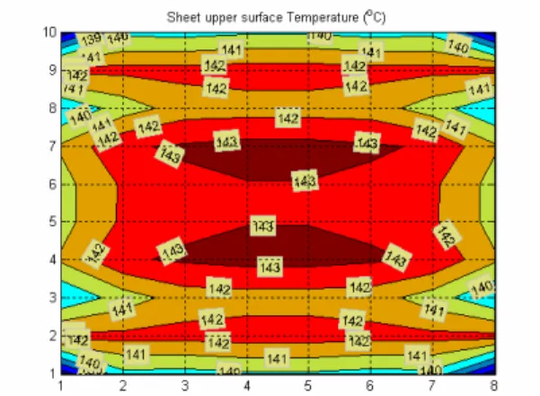
In order to find out the real temperature difference, the optimal heating profiles using Finite Difference Method was applied to heating process analysis code developed in previous study(2). Temperature difference between surface and center was remarkably reduced with satisfying Temperature of Forming Window as shown in Fig.1, Fig. 2, Fig. 3 and Table 1.
5. Conclusion
The analysis model can be simplified to 1-D heat conduction problem when the optimization of heater power distribution to get uniform surface temperature in previous study was acceptable, and the effect of natural convection must be considered(1,2). In order to consider natural convection effect, Finite Difference Method was used, Optimization was carried out under the condition of satisfying Temperature of Forming Window. Verifying the optimal heating profiles by using heating process analysis code developed in previous study, it was found out that the developed method in this study can be used to improve quality of polymer products.
Fig. 1 Time-dependent variation of temperature at each point
Fig. 2 Upper surface temperature distribution
Fig. 3 Lower surface temperature distribution Table 1 Temperature difference between surface and
center
Heating Profile Difference Uniform Heating Profile 15.8℃ Optimum Heating Profile
Using FDM 2.3℃
Reference
(1).Zhen-Zhe Li, Kwang-Su Heo, Jun-Hoo Choi and Seoung-Yun Seol: Optimal Heater Control of Thermoforming using Analytic Solution, Proceeding of
KSME Annual Spring Conference: Thermal Engineering,
pp. 327-330, 2008.
(2).Zhen-Zhe Li, Kwang-Su Heo and Seoung-Yun Seol: A Study of Time-Dependant Optimal Heater Control for Thermoforming using Response Surface Method,
Proceeding of KSME Annual Spring Conference, pp.
3181-3186, 2007.
(3) Jasbir S. Arora: Introduction to Optimum Design, 2nd Edition. McGraw-Hill, 2001. ) 0085 . 3 ( ) ( 0.0310 , t u inp u t q e q = − ) 9972 . 3 ( ) ( 0.0430 , t l inp lt q e q = − 2 1 1 2 x T T T C k t T T i i i p old i i ∆ + − = ∆ − + − ρ c inp q q q= − 2255