Monitoring of Multi-phase Flow using Electrical Impedance Tomography with Level Set-based Method

저작자표시-비영리-변경금지 2.0 대한민국 이용자는 아래의 조건을 따르는 경우에 한하여 자유롭게 l 이 저작물을 복제, 배포, 전송, 전시, 공연 및 방송할 수 있습니다. 다음과 같은 조건을 따라야 합니다: l 귀하는, 이 저작물의 재이용이나 배포의 경우, 이 저작물에 적용된 이용허락조건 을 명확하게 나타내어야 합니다. l 저작권자로부터 별도의 허가를 받으면 이러한 조건들은 적용되지 않습니다. 저작권법에 따른 이용자의 권리는 위의 내용에 의하여 영향을 받지 않습니다. 이것은 이용허락규약(Legal Code)을 이해하기 쉽게 요약한 것입니다. Disclaimer 저작자표시. 귀하는 원저작자를 표시하여야 합니다. 비영리. 귀하는 이 저작물을 영리 목적으로 이용할 수 없습니다. 변경금지. 귀하는 이 저작물을 개작, 변형 또는 가공할 수 없습니다.

Monitoring of Multi-phase Flow using Electrical Impedance

Tomography with Level Set-based Method

Dong Liu

(Supervised by Professor Kyung Youn Kim)

A thesis submitted in partial fulfillment of the requirement for the degree of Master of Science

2011. 06

The thesis has been examined and approved.

Thesis director, Sin Kim, Professor, Department of Nuclear and Energy Engineering

Min Jae Kang, Professor, Department of Electronic Engineering

Kyung Youn Kim, Professor, Department of Electronic Engineering

Date

MAJOR OF ELECTRONIC ENGINEERING FACULTY OF APPLIED ENERGY SYSTEM

GRADUATE SCHOOL JEJU NATIONAL UNIVERSITY

Contents

1. Introduction...1

1.1 Electrical impedance tomography...1

1.2 Shape reconstruction problem...3

1.3 Aims and contents of the thesis ...6

2. Forward problem...7

2.1 Physical model inside the body...7

2.2 Complete electrode model...9

2.3 Numerical solution of forward problem...10

2.4 Jacobian calculation for resistivity change...14

3. Shape reconstruction in EIT...17

3.1 Level set method ...18

3.1.1 Level set formulation for two-phase flow ...18

3.1.2 General multi-phase formulation ...19

3.1.3 Inverse problem using level set method ...21

3.2 Jacobian calculation with level set function...22

3.3 Results and discussion ...24

3.3.1 Numerical results ...24

3.3.2 Experimental results...36

4. Conclusions...40

Summary ...41

초록

전기 임피던스 단층촹영법(EIT)에서는 경계면의 전기적 측정치로부터 대상체 내부의 도전율 또는 유전율에 대한 영상이 얻어진다. 일반적으로, 대상체 주위에 일정한 간격으로 전도성 전극을 부착하고 이 전극들을 통해 소량의 전류를 주입시킨다. 이에 유기되는 전기 신호인 전압을 측정하는데, 이 과정을 여러 다른 전류 패턴들에 대해서 반복 수행한다. 그리고 주입시킨 전류와 측정 전압 데이터를 사용하여, 대상체 내부의 도전율 분포 또는 저항률 분포에 대한 근사치를 얻을 수 있다. 수학적으로, EIT 문제는 비선형이고 부정치성 역문제이다.

본 논문에서는, EIT 에서 level set 방법을 기반으로 한 다상류(multi-phase flow)에 대한 모양 복원(shape reconstruction) 방법을 제안한다. 이 방법의 주요 특징은 서로 다른 도전율 값을 갖는 영역들 사이의 경계를 찾는 역문제를 풀기 위해 협대역(narrowband) level set 방법을 사용하는 것이다. 다상 level set 모델을 사용함에 있어서, 도전율은 두 level set 함수에 의해 주어질 수 있다. 주요 아이디어는 level set 이론을 기반으로, 고차원 함수의 (zero) level set 으로서 모양의 경계(shape interface)를 나타내고 나서 편미분 방정식들의 집합을 푸는 것이다. level set 기반의 기법은 전형적인 픽셀 기반의 접근 방법과 비교해서 몇몇 이점들을 제공한다. level set 전략은 전개 과정 동안 저절로 위상기하학적 병합(topological merging)과 분리(breaking)를 다룬다. 다상의 경우에 대해 적용시키기 위해 level set 방법을 확장하였고, 수치적 데이터와 실험 데이터를 사용하여 제안 알고리즘을 테스트 하였다. 그 결과, 모양 기반의 level set 방법이 픽셀 기반의 영상 방법과 비교해서 더 나은 복원 성능을 보였다.

Chapter 1

1. Introduction

1.1 Electrical impedance tomography

Electrical impedance tomography (EIT) is an imaging technique to view cross-sectional image of

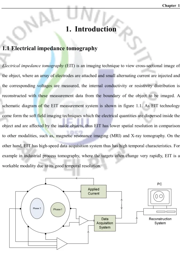
the object, where an array of electrodes are attached and small alternating current are injected and the corresponding voltages are measured, the internal conductivity or resistivity distribution is reconstructed with these measurement data from the boundary of the object to be imaged. A schematic diagram of the EIT measurement system is shown in figure 1.1. As EIT technology come form the soft field imaging techniques which the electrical quantities are dispersed inside the object and are affected by the inside objects, thus EIT has lower spatial resolution in comparison to other modalities, such as, magnetic resonance imaging (MRI) and X-ray tomography. On the other hand, EIT has high-speed data acquisition system thus has high temporal characteristics. For example in industrial process tomography, where the targets often change very rapidly, EIT is a workable modality due to its good temporal resolution.

Figure 1.1 Schematic diagram of EIT system

Many applications of EIT have been developed e.g. for medical purpose. For instance, EIT is useful for monitoring patient lungs because the air has a large conductivity contrast to the other tissues in the thorax (Brown 2001). The most promising clinical application is for lung function monitoring of patients being treated with mechanical ventilation. EIT can resolve the changes in

1.1 Electrical impedance tomography

the distribution of lung volumes between dependent and non-dependent lung regions as ventilator parameters are changed. Also EIT is being investigated in the field of breast imaging as an alternative or complementary technique to mammography and magnetic resonance imaging (MRI) for breast cancer detection (Cherepenin et al. 2001, Cherepenin et al. 2002 and Kerner et al. 2002). In industrial field, EIT has been widely applied to monitor flow processes, multi-phase imaging and monitor mixtures of conductive fluids in vessels or pipes (Jones et al. 1993).

In EIT, an image of the conductivity or resistivity distribution of the object is inferred from surface electrical measurements made on the boundary. Image reconstruction in EIT is a kind of nonlinear optimization problem, which means the solution is obtained iteratively and computed through forward and inverse solvers. In forward problem, the conductivity distribution and the injected current are known and the voltages are computed. In inverse problem, the internal conductivity distribution of the object is estimated based on the measured voltage and injected current data. The physical relationship between the internal conductivity or resistivity and measured boundary voltages is governed by a partial differential equation (PDE) derived from Maxwell equations with an appropriate boundary condition. Methods for reconstruction of EIT images are based on mathematical models that connect the internal conductivity or resistivity distribution to the voltages measurements made on the boundary of the object. In (Cheng et al. 1989) various models were studied, such as continuum, average-gap, shunt and complete electrode model (CEM). In connection with EIT problem these models are referred to as electrode models. It was found that the most accurate and popular model is CEM. This model can take into account the shunting effect of the electrodes and also the contact impedances between the electrodes and the object. In most cases, it is impossible to obtain an analytical solution for the forward problem so a numerical technique such as the finite element method (FEM) can be applied (Jain et al. 1997, Polydorides et al. 2002). The EIT reconstruction methods can be divided into two categories,

stationary and non-stationary imaging. Stationary imaging techniques are used for the case where

the internal conductivity of the object is time invariant within the time taken to acquire a full set of measurement data. In this thesis, reconstruction methods for the stationary cases are considered. In

non-stationary imaging or dynamic imaging technique, which have been introduced to enhance

1.2 Shape reconstruction problem

rapidly. In these dynamic approaches, the time-dependence of the conductivity distribution is taken into account, and a reconstruction is obtained after each current injection. The reduction in current patterns is also made possible by the analysis of current patterns to use only the optimal current patterns in a dynamic scenario. With the evaluation of the norm and power distinguishability, the optimal current pattern can be determined (Isaacson 1990, Gisser et al. 1988). With or without using the optimal current patterns, many dynamic techniques were proposed in which the inverse problem is treated as a nonlinear state estimation problem and the time-varying state is estimated with a suitable reconstruction method, where the Kalman filter (KF) (Vauhkonen 1997, Kim et al. 2001) is the most popular method for tracking the dynamic changes.

1.2 Shape reconstruction problem

Two-phase or multi-phase flow can occur in a variety of industrial applications, such as in condensers, nuclear cooling systems, and fluidised bed sulphide roasters, heat exchangers, and oil pumping for example. The constituents may be gas and liquid, such as air/water or steam/water, gas and solid, as in a fluidised bed. Liquid/liquid immiscible flows occur in oil extraction, where oil mixes with water in the borehole. The phase distribution affects the safety, control and operation of mechanical systems and clinic treatment therefore it is necessary to determine the phase distribution without disturbing the flow field (figure 1.2).

In order to achieve even more voracious measurement information on two-phase flow section, and carry out non-intrusive and non-destructive collecting information, many novel sensor techniques have been applied to the measurement of two-phase flow, such as radiation (Banerjee et al. 1981), laser (Kumar et al. 1995), nuclear magnetic resonance (NMR) (Lynch et al. 1977), ultrasonic (Couthard et al. 1993), and tomography. One kind of attractive technique to measure two-phase flow parameters is a method based on electrical tomography. Such a method uses non-intrusive or non-invasive sensors that are located on the boundary of objects, such as process vessels or pipelines, to reconstruct the spatial distribution of the interfaces among various phases and then form the cross-sectional image of the phase distributions of objects. The electrical tomographic methods applied in two-phase flow measurement such as electrical capacitance tomography (ECT),

1.2 Shape reconstruction problem

electrical resistivity tomography (ERT), and EIT have become popular. For example, ERT system was used to measure the gas–liquid mixture in a stirred vessel (Wang et al. 1999). An ERT system applied to monitor the hydro cyclone operation (Bond et al. 1999). Also measurement parameters of two-phase flow using ERT system has been studied (Dong et al. 2003). A real-time EIT system was used to image the flow of saline through the human vascular system (Brown et al. 1992), EIT system was used to image a volunteer's forearm during resting cardiovascular activity (Halter et al. 2008). In case of multi-phase flow, similar as two-phase flow, EIT can be a promising technique to reconstruct the phase distribution. In many situations, the knowledge of the conductivities of the anomalies is known a priori. The prior information of the conductivities can be used in the inverse algorithm to estimate the size, shape and location of the anomalies. The process of the estimating the phase distribution from the measured voltages made on the boundary is named as shape reconstruction problem. Conductivity of background phase Conductivity of phase 2 Conductivity of phase 1 0

s

1

s

2

s

Figure 1.2 Shape reconstruction of multi-phase flow using EIT

Shape reconstruction has been studied by many researchers and different methods are proposed to represent the shape of the anomalies occurring in flow process (Tamburrino et al. 2003, Kolehmainen et al. 1999). Level set method has emerged recently as an attractive alternative to solve topology optimization problems (Osher et al. 1988). A level set representation can describe concisely the geometric and material boundaries of an anomaly, for example it can be used to represent or identify piecewise constant or piecewise smooth functions of the inclusions (Luminita

et al. 2002, Osher et al. 2001 and Chung et al. 2005). More importantly, it has strong ability to

1.2 Shape reconstruction problem

components. Level set method has become powerful and versatile tool for image processing and computational physics (Luminita et al. 2002, Osher et al. 2001 and Osher et al. 2003), also it has found applications in shape reconstruction and inverse scattering (Dorn et al. 2000, Dorn et al. 2006). More recently, applications of level set method to electrical tomography problems have been proposed. In Ito et al. 2001, using values of Neumann data as well as values of solution in a thin layer along the domain, level set method together with steepest descent method has been employed to solve the inverse conductivity problem. In Soleimani et al. 2006a, narrow band level set method applied in Gauss-Newton method as an inverse algorithm was used to estimate the shape and conductivities of two-phase. In Soleimani et al. 2006b, a similar method as in Soleimani

et al. 2006a was employed using EIT to imaging of the human brain. Most of the work discussed

before are related to the reconstruction of two-phase. In real situations, more than two-phase can exist, therefore, multi-phase reconstruction will provide better visualization of the flow characteristics.

In this thesis, we present shape reconstruction technique based on level set method using EIT. Multi-phase reconstruction is done where the conductivity values of the inhomogeneous background and that of anomalies are known, and the size, shape and location of the anomalies are unknown. Gauss Newton method based on level set method in Soleimani et al. 2006a and multi-phase framework for image segmentation in Luminita et al. 2002 are employed into multi-phase shape reconstruction. In using a multi-phase level set model, we will represent the conductivity by two level set functions. Based on the level set theory, the key idea was to implicitly represent the shape interface as the zero level set of a higher dimensional function, and then solve a set of partial differential equations in the Cartesian coordinate system which contains the shape of this new embedding function. The shape is set as the zero level set of higher dimensional functions, so the computational cost and time will increase. In order to reduce the cost time, we used a narrowband technique to calculate the shape deformation or update. The combination of the narrowband technique and optimization approach results in a computationally efficient and fast method for solving the inverse problem.

1.3 Aims and contents of the thesis

1.3 Aims and contents of the thesis

The aims of this thesis are:

1. To apply level set method for monitoring of multi-phase flow using EIT. 2. To investigate the performance of the proposed algorithm.

3. To evaluate the proposed approach with standard pixel-based Gauss Newton method using numerical and experimental data.

This thesis contains four chapters. Chapter 1 gives a soft introduction about EIT and shape reconstruction in general. The most commonly applied applications and methodology are given in this chapter and an overview of this thesis is given. In chapter 2 the most widely used EIT electrodes model, so-called complete electrode model (CEM), is presented and a finite element method (FEM) is applied to solve the forward problem of EIT. The solution of CEM, that is, the solution of the potential distribution when injected currents and conductivity or resistivity are known, is necessary in the implementation of inverse problem. Also the Jacobian calculation is discussed in this chapter. Chapter 3 constitutes the main part of this thesis, in which the novel shape-based level set method is applied to reconstruct the shape of the flow process. Several numerical simulations and experimental case for multi-phase flow are studied to demonstrate the performance of the proposed method. Finally, the conclusion and guidelines of the future research are summarized in chapter 4.

Chapter 2

2. Forward problem

In order to solve an EIT reconstruction problem, a physical model need to be derived from the prior information, such as measured voltage, injected current, and a conductivity distribution. The equations for the physical model can be derived from Maxwell equations of electromagnetism (Malmivuo et.al. 1995, Doerstling 1995). In this chapter, the so-called complete electrode model (CEM) applied into governing equation with boundary conditions to solve the EIT problem is presented. The numerical solution for CEM is also given. Also Jacobian defined as the rate of change of potential with respect to the conductivity or resistivity is derived.

2.1 Physical model inside the body

Maxwell’s equations in the domain Ω can be written as

E

B

t

¶

Ñ´ =

-¶

(2.1)

D

H

J

t

¶

Ñ´

= +

¶

(2.2)

where E is the electric field, H magnetic field, D electric displacement, B magnetic induction, and

J electric current density.

In case of linear isotropic medium domain Ω, the following equations holds true

D = εE

(2.3)

B = µH

(2.4)

J = σE

(2.5)

where ε is permittivity, µ permeability, and σ conductivity of the medium. Assuming that the injected currents are time harmonic with frequency

w

_{and using the previous equations (2.3-2.5)} we get the following relationships

2.1 Physical model inside the body

_E

_{= %}

_Ee

i tw _(2.6)

i t

B

_{= %}

Be

w _(2.7)

Solving equations (2.1) and (2.2) using equations (2.3) to (2.7), we get

(

)

( )

( )

i t i t i t i t

B

Be

E

t

t

e

B

e

B

iwBe

i

H

t

t

w w w w

_wm

¶

¶

Ñ´ = -

=

-¶

¶

¶

¶

= -

-

= -

-¶

¶

%

%

%

%

(

)

(

)

( )

( )

i t i t i t i t

D

E

Ee

H

J

J

J

t

t

t

e

E

e

E

J i

Ee

J i

E

t

t

w w w w

e

e

e

e

we

we

¶

¶

¶

Ñ´

= +

= +

= +

¶

¶

¶

¶

¶

= +

+

= +

+

¶

¶

%

%

%

%

In EIT, the current density J can be divided into two components, which are so-called ohmic current (

J

0

=

s

E

)and current source (

J

s). The following simplified Maxwell equations can hold true without the oscillatory exponential terms (Somersalo et al. 1992, Ola et al. 1993, Doerstling 1995)

E

i

wm

H

Ñ´ = -

(2.8)

(

)

s

.

H

s we

i

E J

Ñ´

=

+

+

(2.9)

In EIT, some simplifications are made for those equations, such as assuming static conditions, which mean that the effect of magnetic induction which produces an induced electric field is neglected. Also the capacitive effects

i

we

E

in (2.9) is assumed be neglected (Barber et al. 1984, Baker 1989). With these assumptions, the above equations can be simplified as

E

= -Ñ

u

(2.10)

.

s

H

s

E J

Ñ´

=

+

(2.11)

2.2 Complete electrode model

(

s

u

) 0

Ñ × Ñ

=

(2.12) can be obtained for EIT inside the domain. where u = u(x,y), for x,y

Î

Ω

.

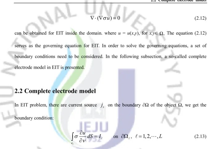
The equation (2.12) serves as the governing equation for EIT. In order to solve the governing equations, a set of boundary conditions need to be considered. In the following subsection, a so-called complete electrode model in EIT is presented.

2.2 Complete electrode model

In EIT problem, there are current source

j

_s on the boundary ∂Ω of the object Ω, we get the boundary condition: e

u

dS

I

s

n

¶

₌

¶

ò

l l on

¶W

l,

l

=

1, 2, , L

L

(2.13) In order to taking convenience on research of CEM, we set the zone between two electrodes by

h

¶W

, and assume that there is no current on

¶W

_h, so we get

s

u

0

n

¶

₌

¶

on

¶W

h (2.14)

In actual application of EIT, we should take account of the imperfect contact between electrode and object, according series connection theorem (see figure 2.1), the real potential of electrode should be the plus of the potential at the object and the contact impedance potential. Described as:

u

u z

s

U

n

¶

+

=

¶

l l

( )

x y

,

Î

e

l,

l

=

1, 2, , L

L

(2.15) where

z

_l is the effective contact impedance between the

l

th electrode and object.

U

_l is the measured boundary potential.

u Ul u zs n ¶ ¶ l

2.3 Numerical solution of forward problem

2.3 Numerical solution of forward problem

In section 2.2, equations set of CEM are obtained, the main goal is to find the potential

( )

,

u x y

on

W

and the voltages

U

_l on the electrodes with the information of the injected

currents, measured boundary voltages and the prior knowledge on the resistivity values. With a small change of governing equation 2.12, and define

F = Ñ

s

u

, then

(

s

u

)

0

Ñ ×F = Ñ × Ñ =

(2.16)

Using a test function V to multiply equation (2.16),we can get

0

V

Ñ ×F =

(2.17) And integrating the equation (2.17) over the object Ω

0

V

dp

W

Ñ ×F

=

ò

(2.18) For

V ds

(

V

)

dp

V

dp

V

dp

¶W W W W

F = Ñ × F

=

Ñ ×F + Ñ ×F

ò

ò

ò

ò

(if ∂Ω is smooth enough)

Then

V

s

uds

V

s

udp

¶W W

Ñ

= Ñ × Ñ

ò

ò

(2.19)

As we know, there is no current on

¶W

_h, thus equation (2.19) can be written that

1 L e

V

s

uds

V

s

udp

= _W

Ñ

= Ñ × Ñ

å ò

ò

l l (2.20)

Furthermore, the equation (2.15) implies

u U

u

z

s

Ñ = -

-

l l (2.21)

Now the equation (2.20) can be written in the form

1

1

(

)

0

L e

u U Vds

u

Vdp

z

s

= W

-

+ Ñ ×Ñ

=

å ò

l

ò

l l l (2.22)

2.3 Numerical solution of forward problem Then 1 1

1

0

L L e e

U

u

Vdp

uVds

Vds

z

z

s

= = W

Ñ ×Ñ

+

å

-

å

=

ò

ò

l

ò

l l l l l l (2.23)

Next, using equation (2.21) into boundary equation (2.13), we can get

1

(

)

e

U

u ds I

z

ò

l

-

=

l l l (2.24)

For

U

_l is a constant parameter, then

1

e e

U

uds

ds I

z

z

-

₊

₌

ò

l

ò

l l l l l Set e

e

=

_ò

ds

l

l

, where

el

is the area of the electrode

l

.

Equation (2.24) becomes

1

e

e

uds

U

I

z

z

-

₊

₌

ò

l l l l l

l

(2.25)

In general, most of the forward problem cannot be solved analytically, thus numerical methods have to be employed. In this thesis, we use the finite element method (FEM) to obtain the numerical solution for the forward problem. In the context of FEM, the domain Ω is discretized into small triangular elements and the finite dimensional approximations are written for the unknown functions. The potential distribution within the object Ω is approximated by the finite sum in the form of

1 N h n n n

u u

u

=

»

=

å

F

(2.26) Also set

V

= F

_m, then equation (2.23) becomes

1 1 1 1

1

(

N _{n n}

)

_m L N _{n n m} L _m

0

n _e n _e

U

u

dp

u

ds

ds

z

z

s

= = = = W

Ñ

å

F

×ÑF

+

å

å

F

F

-

å

F

=

ò

ò

l

ò

l l l l l l (2.27) 1 1 1

1

[

]

0

N L L n n m n m m n e e

U

u

dp

ds

ds

z

z

s

= _W = =

ÑF ×ÑF

+

F F

-

F

=

å

ò

å

ò

å

l

ò

l l l l l l (2.28)

In matrix form, we can write as

, , 1 1

0

N L n m n m n

B u

C U

= =

+

=

å

å

l l l (2.29)

2.3 Numerical solution of forward problem Where , 1 ,

1

1

L n m n m n m e m m e

B

dp

ds

z

C

ds

z

s

= W

=

ÑF ×ÑF

+

F F

= -

F

å

ò

ò

ò

l l l l l l

For equation (2.25), use

1 N h n n n

u u

u

=

»

=

å

F

, it becomes 1

1

N n n n e

e

u ds

U

I

z

=

z

-F

+

=

å

ò

l l l l l

l

1

1

N n n n e

e

u

ds

U

I

z

z

=

-

_F

₊

₌

å

ò

l l l l l

l

Define n,

1

_n e

C

ds

z

-=

ò

F

l l l ,

D

e

z

=

l l

l

, then , 1 N n _n n

C u

D U

I

=

+

=

å

l _{l l l} (2.30) Finally, the following system of linear equations is obtained from the finite element formulation

AX

=

b

uvuuv

v

(2.31) Where T

B

C

A

C

D

æ

ö

= ç

÷

è

ø

,

u

X

U

æ ö

= ç ÷

è ø

,

0

b

I

æ ö

= ç ÷

è ø

That is

0

T

B

C

u

C

D U

I

æ

öæ ö æ ö

=

ç

÷ç ÷ ç ÷

è ø è ø

è

ø

(2.32)

In EIT, the potentials at the electrodes can be expressed in a matrix form as

1 2

1

1

1

1 0

0

0

1

0

0

0

1

h L

U

U

U

NU

U

æ

ö

æ

_{öç ÷}

ç

_-

_{÷ç ÷}

ç

_{÷ç ÷}

ç

÷

=

-

_ç

_÷

=

ç

_{÷ç ÷}

ç

_{÷ç ÷}

ç

_{- ç}

÷

_÷

è

_{øè ø}

L

L

M

L

M

M

M

O

M

L

2.3 Numerical solution of forward problem Where

(

_{1 2 1}

)

1

1

1

1 0

0

, , ,

0

1

0

0

0

1

L

N

n n

n

-æ

ö

ç

_-

÷

ç

÷

ç

÷

=

=

-ç

÷

ç

÷

ç

_-

÷

è

ø

L

L

L

L

M

M

O

M

L

,

U

=

(

U

₁

U

₂

L L

U

_L

)

T

Now, equation (2.32) can be written as

0

T

u

B

C

C

D

NU

I

æ

ö

æ

ö

æ ö

=

ç

÷

ç

÷

ç ÷

è ø

è

øè

ø

Using matrix transform, we can get

0

T T T T

u

B

CN

N C

N DN

U

N I

æ ö æ

ö

æ

ö

=

ç ÷ ç

÷

ç

÷

è

ø

è ø

è

ø

Set

(

)

1 2 1 2 1 3 1

1

1

1

1 0

0

,

, ,

0

1

0

0

0

1

T T T L L

I

I

I

N I

I

I I

I

I

I

I

æ ö

æ

ö

ç ÷

ç

_-

÷

ç ÷

ç

÷

ç ÷

ç

÷

=

=

-

=

-

-

-ç ÷

ç

÷

ç ÷

ç

÷

ç

_-

÷ ç ÷

è

ø è ø

L

L

%

_L

_M

_L

M

M

M

O

M

L

Then

0

T T T

u

B

CN

N C

N DN

U

I

æ ö æ ö

æ

ö

=

ç ÷ ç ÷

ç

÷

è

øè ø è ø

%

(2.33)

Solving the equation (2.31) or equation (2.33) as

X

₌

A b

-1 _{, the approximation solution for the} forward problem is obtained.

The elements of the other matrices in matrix

A

are

( )

1

1

1

B ,

_{i j} L _{i j} e

i j

d

dS

z

j

j

j j

r

= W

=

ò

Ñ ×Ñ

W +

å

ò

l l l ,

i j

,

=

1, 2, ,

L

N

(2.34)

( )

,

1

j i j e

C i j

dS

z

j

= -

ò

,

i

=

1,2, ,

L

N

,

j

=

1, 2, ,

L

L

(2.35)

( )

,

j ij j ij i e i

e

D i j

dS

z

z

d

d

=

_ò

=

0

j j

i

j

e

i

j

z

¹

ì

ï

= í

₌

ï

î

i j

,

=

1, 2, ,

L

L

(2.36)

2.4 Jacobian calculation for resistivity change

2.4 Jacobian calculation for resistivity change

Jacobian is defined as the rate of change of potential with respect to the conductivity or resistivity, the resulting matrix is defined as Jacobian matrix. In the applications of EIT, a set of current patterns should be used. Even with the consideration of the current patterns, the expression of the above equation will not be altered if the resistivity and the contact impedance do not depend on the current pattern. If

P

is the number of the current patterns,

u

_ÎÂ

N P´ _,

_U

_ÎÂ

(L- ´1)P_{, and}

~

L P

I

_ÎÂ

´ _.

In some cases, the voltages are measured only at some selected electrodes, not every electrode. Also, the selected electrodes may be different at each current pattern. The measured voltages at the measurement electrodes

U

can be obtained as

T h T E P

U

=

M U

=

M NU

ÎÂ

´ (2.37)

where,

E

is the number of the measurement electrodes and

M

_ÎÂ

L E´ _{is the measurement} matrix. The element

M

( , )

l

p

is set to ‘1’ if the

l

-th electrode is measured at the

p

-th current pattern and otherwise set to zero. Furthermore,

U

h can be extracted directly from

X

by

introducing the extended mapping matrix

N

~ ~

( 1)

(0, )

L N L

N

₌

N

_ÎÂ

´ + - _and

_U

h

₌

_{N X}

~ _(2.38)

where

0

_ÎÂ

L N´ _{. Therefore, we have}

~ ~

T h T

U

=

M U

=

M N X

=

M X

_(2.39)

where the extended measurement matrix is defined as

~ ~

( 1)

T E N L

M

=

M N

ÎÂ

´ + - _{. (2.40)}

The Jacobian defined as the relative change of the measured voltage at the

l

-th measurement electrode at the

p

-th current pattern (

U

ˆ

_lp) with respect to the change of the conductivity or resistivity of the

m

-th pixel (

r

_m), that is

2.4 Jacobian calculation for resistivity change

ˆ

p pm m

U

J

r

¶

=

¶

l l (2.41) or in a matrix form 1 1 1 1 1 1 1 2 1 1 1 2 2 2 1 2 1 1 1 1 2 2 2 2 1 1 1 1 2 2 2 2 1 2 1 2

ˆ

ˆ

ˆ

ˆ

ˆ

ˆ

ˆ

ˆ

ˆ

ˆ

ˆ

ˆ

ˆ

ˆ

ˆ

ˆ

ˆ

ˆ

M M E E E M M E E E M P P P E E E M

U

U

U

U

U

U

U

U

U

J

_U

_U

_U

U

U

U

U

U

U

r

r

r

r

r

r

r

r

r

r

r

r

r

r

r

r

r

r

æ

¶

¶

¶

ö

ç

÷

¶

¶

¶

ç

÷

ç

_¶

_¶

_¶

÷

ç

÷

¶

¶

¶

ç

÷

ç

÷

ç

÷

ç

_¶

_¶

_¶

÷

ç

÷

¶

¶

¶

ç

÷

ç

= ¶

_ç

¶

¶

ç ¶

¶

¶

ç

ç

ç ¶

¶

¶

ç

¶

¶

¶

ç

ç

ç

ç ¶

¶

¶

ç

¶

¶

¶

è

ø

L

L

M

M

M

M

L

L

M

M

M

M

L

M

M

M

M

L

÷

÷

÷

÷

÷

÷

÷

÷

÷

÷

÷

÷

_(2.42)

where

M

is the number of pixels (meshes). The Jacobian matrix can be obtained from the derivative of the system of equation

AX

=

b

(2.43)

and the expression

~ ~ T h T

U

=

M U

=

M N X

=

M X

(2.44) That is,

(

)

1 ~ ~ ~ 1 m m m m

U

X

A

M

M

A b

M

b

r

r

r

r

-¶

¶

¶

¶

=

=

=

¶

¶

¶

¶

1 1 1 1 m m m

A

A

A

b

A

A b

A

X

r

r

r

-- -

-¶

¶

¶

= -

=

-¶

¶

¶

~ ~ ~ 1

₍

1

₎

1 T T T T T m m m m

U

A

A

A

M A

X

A

M

X

A M

X

r

r

r

r

-

æ

-

ö

æ

-

ö

¶

¶

¶

¶

= -

= -

_ç

_÷

= -

_ç

_÷

¶

¶

_è

_ø

¶

_è

_ø

¶

(2.45)

2.4 Jacobian calculation for resistivity change

pseudo-resistance matrix defined as

~ ~

1 T (N L 1) E

R

=

A M

-

ÎÂ

+ - ´ (2.46) is given we can calculate the Jacobian matrix. The pseudo-resistance matrix can be easily obtained during the solution of the system equation

~ ~ T

A R X

æ

_ç

ö = ç

_÷

æ

M

b

ö

_÷

è

_{ø è}

_ø

(2.47) or ~ 1 ~ ~ 2

0

0

T T

R

u

A

N M

N b

R

U

æ

_{ö æ}

_ö

ç

_{÷ = ç}

_÷

ç

_{÷ è}

_ø

è

ø

(2.48) where ~ ~ 1

(1: ,:)

N E

R

=

R

N

ÎÂ

´ and

R

~2

=

R N

~

(

+

1:

N L

+ -

1,:)

ÎÂ

(L- ´1) E (2.49) The derivative of the stiffness matrix with respect to the resistivity is

0

0

0

m m

B

A

_r

r

¶

æ

ö

¶

_ç

_¶

_÷

= ç

÷

¶

_ç

_÷

è

ø

(2.50) Therefore, we have ~ ~ ~ ~ 1 1 2 1 ~ ~ 2

0

0

0

0

T T T T m m m m

B

_u

B

u

R

U

B

R

R

R

u

U

R

r

r

r

r

¶

¶

æ

ö

æ

ö

æ

ö

_{æ ö}

_æ

_ö

¶

_{= -}

_ç

_{÷ ¶}

_ç

_÷

_{ç ÷}

_{= -}

_ç

_¶

_÷

_{= -}

¶

ç

÷

ç

÷

ç

÷

ç

÷

ç ÷

¶

_ç

_÷

_{è ø}

_è

_ø

_ç

_÷

¶

è

_{ø è}

ø

è

ø

(2.51)

in which the term

( )

,

m

B i j

r

¶

¶

can be calculated as

( )

2

,

1

m i j m m

B i j

d

j

j

r

r

_W

¶

= -

Ñ ×Ñ

W

¶

ò

,

i

,

j

=

1

,

2

,

L

,

N

(2.52)

where

j

_i ,

j

_j are basis functions and Wm is the element with which the derivative is

Chapter 3

3. Shape reconstruction in EIT

In EIT, the conductivity or resistivity distribution of the object is inferred from surface voltage measurements made on the boundary and the injected current data. Image reconstruction in EIT is a kind of nonlinear optimization problem, which means the solution is obtained iteratively and computed through forward and inverse solvers. The physical relationship between the internal conductivity or resistivity and measured boundary voltages is governed by a partial differential equation derived from Maxwell Equations with an appropriate boundary condition. For solving the nonlinear system equations, lots of classical method are applied to the impedance reconstruction (Li et al. 2004, Wang et al. 2004), such as modified Newton-Raphson method (mNR), Landweber method (LW), and Differential Evolution algorithm (DE). Recently, various methods that have been proven successful in image processing have also found their way to help solving electrical tomography problems. In this chapter, shape reconstruction based on level set method using EIT is presented. Multi-phase reconstruction is done where the conductivity values of the inhomogeneous background and that of anomalies are known, and the size, shape and location of the anomalies are unknown. Gauss-Newton method based on level set method in Soleimani et al. 2006a and multi-phase framework for image segmentation in Luminita et al. 2002 are employed to monitor the process of multi-phase flow. In using a multi-phase level set model, the conductivities distribution can be presented by two level set functions. Based on the level set theory, the inverse boundary problem is to find a level set function which can implicitly represent the conductivity distribution, and then solve a set of partial differential equations in the Cartesian coordinate system which contains the shape of this new embedding function to minimize the mismatch between the measured and calculated data. As the shape is described by the zero level set of higher dimensional functions, so the computational cost and time will increase. To improve the level set reconstruction process, a narrowband technique applied to calculate the shape deformation or update. The combination of the narrowband technique and optimization approach results in a computationally efficient and fast method for solving the inverse problem.

3.1 Level set method

3.1 Level set method

3.1.1 Level set formulation for two-phase flow

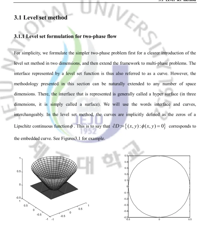
For simplicity, we formulate the simpler two-phase problem first for a clearer introduction of the level set method in two dimensions, and then extend the framework to multi-phase problems. The interface represented by a level set function is thus also referred to as a curve. However, the methodology presented in this section can be naturally extended to any number of space dimensions. There, the interface that is represented is generally called a hyper surface (in three dimensions, it is simply called a surface). We will use the words interface and curves, interchangeably. In the level set method, the curves are implicitly defined as the zeros of a Lipschitz continuous function

f

. This is to say that

¶ =

D

:

{

( , ) : ( , ) 0

x y

f

x y

=

}

corresponds to the embedded curve. See Figures3.1 for example.

-1 -0.5 0 0.5 1 -1 -0.5 0 0.5 1 -0.5 0 0.5 1 -0.5-0.5 0 0.5 -0.4 -0.3 -0.2 -0.1 0 0.1 0.2 0.3 0.4 0.5

Figure 3.1 A circular contour embedded by a level set function.

If D is the inclusion with conductivity

s

_int embedded in a background

W

with conductivity

ext

s

, then the embedded curve, which is the boundary

G = ¶

D

of the inclusion, can be given by the zero level set

{

}

:

( , ) : ( , ) 0

D

x y

f

x y

¶ =

=

(3.1) where the conductivity distribution of each point will be

3.1.1 Level set formulation for two-phase flow

{

}

{

}

int

( , ) : ( , ) 0

( , )

( , ) : ( , ) 0

ext

x y

x y

x y

x y

x y

s

f

s

s

f

<

ì

= í

_>

î

(3.2)

If we add some perturbation on the level set function, which will lead in the change of the shapes automatically. This relationship is used in the level set technique when constructing updates to a given level set function such that the shapes are deformed in a way which reduces a given cost functional. We assume a continuous velocity field

v t

( )

whose restriction onto the curve represents the velocity of the curve, and then at least locally in time, the evolution can be described as a Hamilton-Jacobi-type equation

( )

0

v t

t

f

_f

¶

₊

_{Ñ =}

¶

(3.3)

Here

v t

( )

is a velocity function of evolving contours in their outward direction. we assume the velocity field is regular enough smooth that the basic structure of shape D remains preserved during this evolution. Meantime we assume that

Ñ

f

is well defined and nonzero along the shape boundary represented by a smooth level function

f

( , )

x y

. For solving equation (3.3), usually an approach of steepest descent flow can be applied. See for example (Burger 2001, Ito et

al. 2001).

3.1.2 General multi-phase formulation

In this subsection, the shape parameterization using level set method is presented. With

m

level set functions

(

f f f

1

, , , ,

2 3

L

f

K

)

, we can represent up to

2

m

distinct regions of the form

{

}

1 0

m j j= ± >f

I

(Luminita et al. 2002), and each may be used to represent one phase. For simplicity of presentation, we assume Ω contains three different regions (Figure 3.2) which did not have overlapping and vacuum state with piecewise constant conductivities

s

=

( , ,

s s s

_{0 1 2}

)

, where

0

s

,

s

₁ and

s

₂ are three positive real numbers. In association with the three regions given by the two level set functions

f

=

(

f

₁

( , ), ( , )

x y

f

₂

x y

)

through the representation of the interior conductivity distribution

s

( , )

x y

in Ω as follows.

3.1.2 General multi-phase formulation

0

H

( ) ( )

1

H

2 1

(1

H

( )) ( )

1

H

2 2

(1

H

( )) ( )

2

H

1

s s

=

f

f

+

s

-

f

f

+

s

-

f

f

(3.4)

where H(x) is the Heaviside function, namely

( ) 1

0, ( ) 0

0.

H x

=

for x

³

H x

=

for x

<

(3.5) and

f

=

(

f

₁

( , ), ( , )

x y

f

₂

x y

)

is the level set function satisfying

{

}

{

}

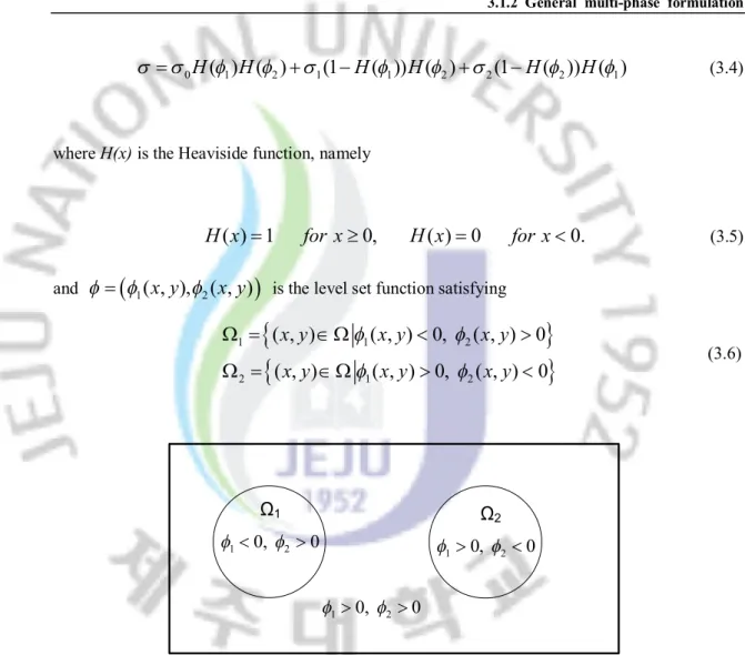
1 1 2 2 1 2

( , )

( , ) 0, ( , ) 0

( , )

( , ) 0, ( , ) 0

x y

x y

x y

x y

x y

x y

f

f

f

f

W =

Î W

<

>

W =

Î W

>

<

(3.6) Ω1 Ω₂ 1 0, 2 0

f

<

f

> 1 0, 2 0

f

>

f

< 1 0, 2 0

f

>

f

>

Figure 3.2 Example of partition of the domain in regions with boundaries represented via two level set functions

Then we can write

1

( )

2

( )

1 2

( )

1

( )

2

g

H

g

H

s

f

f

f

f

Ñ =

×Ñ

+

×Ñ

(3.7) Where 1 2 0 1 2 2 2 2 1 0 2 1 1 1

( ) (

) ( )

(1

( ))

( ) (

) ( )

(1

( ))

g

H

H

g

f

f

=

=

s

s

-

-

s

s

H

f

f

+

+

s

s

-

-

H

f

f

(3.8)

Let

G

j

(

j

=

1, 2

)

be the interface between two different regions, which is also a boundary of the

3.1.3 Inverse problem using level set method

{

}

:

( , ) : ( , ) 0

j

x y

f

j

x y

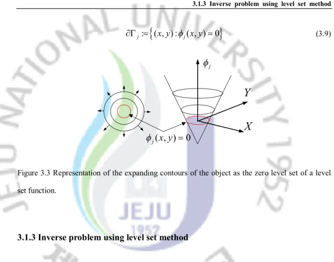
¶G =

=

(3.9)

X

Y

( , ) 0

j

x y

f

=

j

f

Figure 3.3 Representation of the expanding contours of the object as the zero level set of a level set function.

3.1.3 Inverse problem using level set method

If we change the level set function by a small distance, we assume the update is sufficiently smooth, such that the basic structure of the shape remains preserved. Then we move the shapes accordingly. This idea is used in the level set technique when constructing updates to a given level set function such that the shapes are deformed in a way which reduces the objective function. As given in Soleimani et al. 2006a, the Gauss-Newton update for level set function can be written as follows 2 1 2 * 1

(

) [

(

( ))

(

)]

T T T T n n

J J

n n

R R

J V G

n n

R R

n

f

f

l

a

-

f

a

f f

+

=

+

+

-

-

-

(3.10)

Here

J

_nis the Jacobian calculated with

f

_n being the level set function (detail of the Jacobian calculation will be discussed in the next section), V and

G

( )

f

_n are the vector of measured and calculated voltages.

l

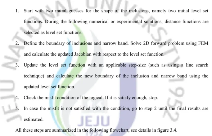
is the time step size for the current update and R is a regularization matrix. To improve the level set reconstruction process, a narrowband technique applied to calculate the shape deformation or update. Here the narrow band means the area that includes elements sharing nodes with the boundary and its neighbors. It was able to reduce the number of elements taking part in the reconstruction process making it better conditioned. The level set-based reconstruction algorithm steps applied to multi-phase case are as follows:

3.2 Jacobian calculation with level set function

1. Start with two initial guesses for the shape of the inclusions, namely two initial level set functions. During the following numerical or experimental solutions, distance functions are selected as level set functions.

2. Define the boundary of inclusions and narrow band. Solve 2D forward problem using FEM and calculate the updated Jacobian with respect to the level set function.

3. Update the level set function with an applicable step-size (such as using a line search technique) and calculate the new boundary of the inclusion and narrow band using the updated level set function.

4. Check the misfit condition of the logical. If it is satisfy enough, stop.

5. In case the misfit is not satisfied with the condition, go to step 2 until the final results are estimated.

All these steps are summarized in the following flowchart, see details in figure 3.4.

start Forward Solver i=0 Initial guess Calculate L.S function Find the boundary of the shape =0 Update conductivity matrix FEM Solver Update Jacobian matrix Shape optimization Φi+1=f(Φi) Define step size If i< iteration number i=i+1 Yes

Final shape End

No

Figure 3.4 Flowchart of level set-based reconstruction algorithm.

3.2 Jacobian calculation with level set function

The Jacobian quantifies the sensitivity of the voltage measurements due to changes of the level set function, as an adaptive parameter in particular, the element conductivity changes. In this section,

3.2 Jacobian calculation with level set function

a formula for the voltage sensitivity

n

U

f

¶

¶

is derived, and we describe how this quantity is

assembled into each component of the Jacobian.

A change in the level set function of an element

k

requires the calculation of

k k k

U

U

J

s

f

s

f

¶

¶

¶

=

=

×

¶

¶

¶

(3.11) where 0

H

( ) ( )

1

H

2 1

(1

H

( )) ( )

1

H

2 2

(1

H

( )) ( )

2

H

1

s s

=

f

f

+

s

-

f

f

+

s

-

f

f

Then the following relationships will be hold true

1 1 0 1 2 1 1 0 1 1

[ ( ( )

( ))

( )]

(

) ( )

U

J

U

H

U

s

s

f

s d f

f

s d f

s

s

s d f

s

¶

¶

=

×

¶

¶

¶

=

×

×

-¶

¶

=

×

-¶

(3.12) and 2 2 0 2 1 2 2 0 2 2

[ ( ( )

( ))

( )]

(

) ( )

U

J

U

H

U

s

s

f

s d f

f

s d f

s

s

s d f

s

¶

¶

=

×

¶

¶

¶

=

×

×

-¶

¶

=

×

-¶

(3.13)

In the above,

d

( )

x

denotes the Dirac function. Also from the previous chapter we can get ~ ~ ~ ~ 1 1 2 1 ~ ~ 2

0

0

0

0

T T T T

B

_u

B

R

u

U

B

R

R

R

u

U

R

s

s

s

s

¶

¶

æ

ö

æ

ö

æ

ö

_{æ ö}

_æ

_ö

¶

_{= -}

_ç

_÷

_ç

_÷

_{ç ÷}

_{= -}

_ç

_÷

_{= -}

¶

¶

ç

÷

¶

ç

÷

ç

÷

ç

÷

ç ÷

¶

_ç

_÷

_{è ø}

_è

_ø

_ç

_÷

¶

è

ø è

ø

è

ø

(3.14) and m i j

B

d

j

j

s

_W

¶

_{= Ñ ×Ñ}

_W

¶

ò

(3.15)

3.3 Results and discussion

3.3 Results and discussion

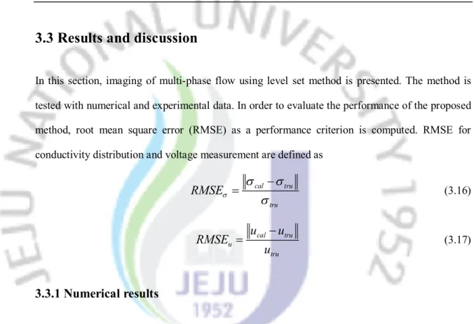
In this section, imaging of multi-phase flow using level set method is presented. The method is tested with numerical and experimental data. In order to evaluate the performance of the proposed method, root mean square error (RMSE) as a performance criterion is computed. RMSE for conductivity distribution and voltage measurement are defined as

cal tru tru

RMSE

s

s

s

s

-=

(3.16) cal tru u tru

u

u

RMSE

u

-=

(3.17)

3.3.1 Numerical results

In this section, the numerical results obtained using level set methods are proposed. We carried out extensive computer simulations with synthetic data to illustrate the reconstruction performance of the proposed algorithm. In order to avoid the so-called ‘inverse crime’, two different finite element meshes are used for forward and inverse problem. A fine mesh (radius of 14 cm) with 3809 nodes and 7306 triangular elements is used in forward solver to generate the boundary voltage data. A coarse mesh with 985 nodes and 1840 triangular elements are used in inverse solvers to reconstruct the shape, location and size of the targets, see figure 3.5.

-15 -10 -5 0 5 10 15 -15 -10 -5 0 5 10 15 -15 -10 -5 0 5 10 15 -15 -10 -5 0 5 10 15 (a) (b)

3.3.1 Numerical results

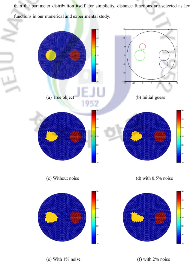
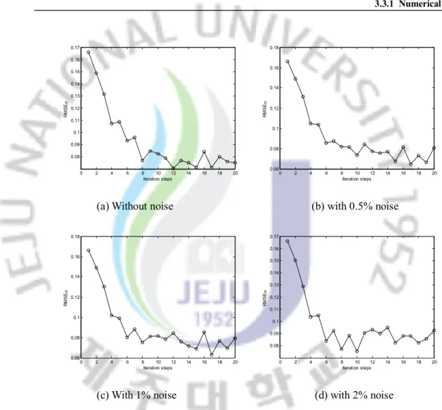
In the first numerical example below, in figure 3.6 the background conductivity is set to 50mS/cm and the conductivity of the inclusions are set to 25mS/cm and 20mS/cm, respectively. With two different circles initial guess, solid line represents the true boundary, while the dashed line shows the initial guess, see figure 3.6(b), the level set method was able to identify the position and a relatively accurate shape of the inclusions. To simulate with actual conditions, Gaussian noise with S.D up to 2% of the corresponding computed voltage are added to the computed data. Reconstructed images of resistivity distribution without or with noise cases are shown in figure 3.6. Two criteria of the performance during the reconstruction are shown in figure 3.7 and figure 3.8, respectively.

In the next two examples (figure 3.9 and figure 3.12), we attempt to reconstruct two objects which are produced probability in industrial process tomography. Considering the actual conditions, Gaussian noise with S.D of 0.5%, 1% and 2% of the corresponding calculated voltage are added to the simulated data. The level set method was able to separate the inclusions clearly, and also identify the position and a good amount of details of the inclusions, see details in figure 3.9 and figure 3.12. The RMSE values of conductivity distribution during the shape reconstruction process are shown in figure 3.10 and figure 3.13, respectively. The RMSE plots of the voltage measurements of case 2 is shown in figure 3.11. The evolution of the shape during the level set reconstruction of case 4, in which inclusions are located relatively close to each other, are shown in figure 3.14. It is interesting to find that the two inclusions could be clearly imaged in the level set-based reconstruction. In case of using a standard regularized pixel-based method, it is difficult to separate those two inclusions. The RMSE value of conductivity distribution and voltage during the shape reconstruction process are shown in figure 3.15. In order to evaluate the performance of level set method, a comparison between level set method and modified Newton-Raphson method is studied in figure 3.16, in which different examples using simulation data are considered. It was found that level set method can easily separate two or more objects which are close to each other and mNR has a poor reconstruction in these cases. The results of level set-based reconstruction using narrow band technique largely depend on the choice of the regularization parameter α and initial guess, here the regularization parameter α not only take charge of the regularization function but also the smooth function. With a choice of α = 0.05, we were able to recover the true

3.3.1 Numerical results

shape at noise level up to 2% with a quite accurate result. The optimal choice of initial guess is a very interesting problem as the level set function has a different significance for the reconstruction than the parameter distribution itself, for simplicity, distance functions are selected as level set functions in our numerical and experimental study.

20 25 30 35 40 45 50 -15 -10 -5 0 5 10 15 -15 -10 -5 0 5 10 15

(a) True object (b) Initial guess

20 25 30 35 40 45 50 20 25 30 35 40 45 50

(c) Without noise (d) with 0.5% noise

20 25 30 35 40 45 50 20 25 30 35 40 45 50

(e) With 1% noise (f) with 2% noise

Figure 3.6 True image of resistivity distribution, initial guess (solid line represents the true boundary, while the dashed line shows the initial guess) and final level set reconstruction for case 1 with or without noise.

3.3.1 Numerical results 0 2 4 6 8 10 12 14 16 18 20 0.08 0.09 0.1 0.11 0.12 0.13 0.14 0.15 0.16 0.17 Iteration steps R M S E s 0 2 4 6 8 10 12 14 16 18 20 0.06 0.08 0.1 0.12 0.14 0.16 0.18 Iteration steps R M S Es

(a) Without noise (b) with 0.5% noise

0 2 4 6 8 10 12 14 16 18 20 0.06 0.08 0.1 0.12 0.14 0.16 0.18 Iteration steps R M S E s 0 2 4 6 8 10 12 14 16 18 20 0.08 0.09 0.1 0.11 0.12 0.13 0.14 0.15 0.16 0.17 Iteration steps R M S Es

(c) With 1% noise (d) with 2% noise