1. INTRODUCTION
These days, many systems need quiet environment for operation without vibration or oscillation. Vibration is undesired disturbance source to the system accuracy, in particular, of the optics and antenna on spacecraft. When a reaction wheels (RW) or control momentum gyros (CMG) control spacecraft attitude, vibration inevitably occurs and degrades the performance of sensitive devices. Therefore, vibration should be controlled or isolated for missions such as Earth observing, broadcasting and telecommunication between antenna and ground stations. Here we attempt to adopt the adaptive vibration controller.
Adaptive controller is that its parameters are on-line adjustable. A number of algorithms have been developed in implementations of adaptive vibration controllers. A typical approach to adaptive vibration control is to feed an error signal through an appropriate filter and apply the resulting signal to a plant. Coefficients of the filter are tuned automatically by an adaptive algorithm to achieve best vibration reduction. Elliott, Stothers and Nelson presented an algorithm to adapt coefficients of an array of finite impulse response (FIR) filters, whose outputs were linearly coupled to another array of error detection points to minimize mean square error signals.[1] Eriksson, Allie, and Greiner investigated the use of IIR adaptive filters in adaptive vibration controls.[2] Baumann studied the potential of an adaptive feedback approach to structural vibration suppression.[3] The filtered-x least mean squares (FLMS) algorithm was derived by Widrow.[4] The adaptation of the weight coefficients involves use of the filtered reference signal vector. The filtered-x least mean squares (FLMS) algorithm requires the reference signal.
In this paper, adaptive notch filter (ANF) finds the disturbance frequency and the reference signal in FLMS is generated by the notch frequency. An adaptive notch filer using the sensor output signal to exactly estimate the actual disturbance frequency could be considered. The design parameters of the notch filter are updated continuously using recursive least square (RLS) algorithm. Therefore, the adaptive FLMS algorithm is applied to the vibration
suppressing experiment without reference sensor. Adaptive vibration controllers are good candidates for problems where parameters of a plant are unknown or there are uncertainties in a system. Parameters of adaptive controllers are adjusted on-line to achieve the best performance.
Due to these characteristics, the FLMS using ANF is a good method to attenuate the spacecraft vibration. For the spacecraft, accuracy requirement in attitude pointing is continuously being heighten. In space there could be many disturbance sources such as solar radiation pressure, and aerodynamic forces which inhibit high accuracy. The main source of spacecraft vibration is the RW or CMG. This disturbances are in the high frequency domain above 10Hz and they degrade spacecraft pointing performance and communication accuracy to the ground station. Therefore, it is targeted to apply this study to the vibration isolation of space applications and shows the experimental results of an adaptive vibration controller.
2. JITTER SUPPRESSION DEVICE
The vibration isolation device to which an adaptive vibration control algorithm is adopted has 3-DOF, one translational and two rotational motions as shown in Fig. 1, and associated dynamics equations are derived. Figure 2 shows the coordinate definition of 3-DOF jitter suppression device. The origin of the coordinate is located at the
center-of-gravity (CG) of the upper plane. w denotes
z-directional translation of CG. φ and θ are the rotational motion in the x and y-axis of the CG. w w w1, 2, 3 which denote
z-axis translational motion of each strut are controlled by three actuators that are connected parallel to the strut. Their relations are 1 1 2 2 4 3 3 4 sin sin sin sin sin w w L w w L L w w L L θ θ φ θ φ = − = + − = + +
(1)
Study on Satellite Vibration Control Using Adaptive Algorithm
Choong-Seok Oh
*, Se-Boung Oh , and Hyochoong Bang
*Division of Aerospace Engineering, KAIST, Daejon, Republic of Korea (Tel : +82-42-869-3789; E-mail: {csoh,sboh,hcbang}@fdcl.kaist.ac.kr)
Abstract: The principal idea of vibration isolation is to filter out the response of the system over the corner frequency. The
isolation objectives are to transmit the attitude control torque within the bandwidth of the attitude control system and to filter all the high frequency components coming from vibration equipment above the bandwidth. However, when a reaction wheels or control momentum gyros control spacecraft attitude, vibration inevitably occurs and degrades the performance of sensitive devices. Therefore, vibration should be controlled or isolated for missions such as Earth observing, broadcasting and telecommunication between antenna and ground stations. For space applications, technicians designing controller have to consider a periodic vibration and disturbance to ensure system performance and robustness completing various missions. In general, past research isolating vibration commonly used 6 degree order freedom isolators such as Stewart and Mallock platforms. In this study, the vibration isolation device has 3 degree order freedom, one translational and two rotational motions. The origin of the coordinate is located at the center-of-gravity of the upper plane. In this paper, adaptive notch filter finds the disturbance frequency and the reference signal in filtered-x least mean square is generated by the notch frequency. The design parameters of the notch filter are updated continuously using recursive least square algorithm. Therefore, the adaptive filtered-x least mean square algorithm is applied to the vibration suppressing experiment without reference sensor. This paper shows the experimental results of an active vibration control using an adaptive filtered-x least mean squares algorithm.
Fig. 1 3-DOF jitter suppression device X Y L4 W1 W2 Z L3 L1 W3 L2 b L4 X Z Y φ θ
Fig. 2 Coordinate definition for the 3 DOF jitter suppression device
A spring, a damper, and an actuator are installed in each strut. The k , i c , and (i F ii =1,2,3) are spring coefficient, damping coefficient, and actuator force, respectively. The force and moment equations are derived as
1 1 2 2 3 3 1 1 2 2 3 3 1 2 3 ( sin ) ( sin ) ( sin ) ( sin ) ( cos ) ( cos ) mw k w L k w L k w L c w L c w L c w L F F F θ θ θ θ θ θ θ θ = − − − + − + − − − + − + + + + && & & & & & &
(2)
1 1 1 2 2 2 3 3 3 1 1 1 2 2 2 3 3 3 1 1 2 2 3 3 ( sin ) ( sin ) cos ( sin ) ( cos ) ( cos ) ( cos ) y I k w L L k w L L k w L L c w L L c w L L c w L L F L F L F L θ θ θ θ θ θ θ θ θ θ θ = − − + − + − − − + − + + − − && & & & & & &(3)
2 4 4 3 4 4 3 4 4 3 4 4 2 4 3 4 ( sin ) ( sin ) cos +c ( cos ) ( cos ) + z I k w L L k w L L w L L c w L L F L F L φ φ φ φ φ φ φ φ = − − + − − + − && & & & &(4)
3-DOF dynamics are expressed in nonlinear equations from the relationship among w , φ, and θ.
3. ADAPTIVE VIBRATION CONTROLLER
In this section, the designed adaptive vibration controller is presented. The adaptive vibration controller is composed of an adaptive notch filter and a least mean square filter.
3.1 Adaptive notch filter (ANF)
The multi mode notch filter of a ARMA structure is required to compute matrix calculation. Hence, it is difficult to apply it to real time system for multiple sinusoids signal case. To reduce the computation time, the cascade of second-order notch filters is designed as shown in Fig. 3. When the number of the spacecraft jitter frequencies to be rejected is p, each notch frequency is determined by each second-order notch filter in the cascade.
1 ( ) k H z− 1 1( ) H z− ( )1 p H z−
( )
u n
( ) k y n 1( ) k y n− 1( ) y n y np−1( ) y np( )Fig. 3 Cascade of second-order notch sections Rao and Kung[5] proposed the following form of a second order notch filter in the z-domain
1 1 1 1 1 1 1 1 1 1 2 2 1 1 1 2 2 2 1 1 (1 )(1 ) ( ) (1 )(1 ) 1 2 cos = 1 2 cos j j k r e zj r e jz H z r e z r e z r z r z r z r z φ φ φ φ ρ ρ φ ρ φ ρ − − − − − − − − − − − − − = − − − + − +
(5)
However, the filter architecture in Eq. (5) is not most appropriate to apply the adaptive notch filter algorithm, so the following notch filter for adaptation has been proposed by Regalia[6]: 1 2 1 1 2 0 1 1 1 (1 ) ( ) 1 (1 ) k a b z bz H z z z β β β − − − − − + + + = + + +
(6)
In order to match Eq. (5) with Eq. (6), it should be satisfied that 0 1 2 1 (1 ) a(1 b) b β β ρ β ρ + = + =
(7)
This can be reduced to
0 (1 2 ) 1 a b b ρ β ρ + = +
(8)
For implementation of adaptive notch filters, the number of parameters to be adapted should be maintained minimum. If we assume ρis equal to 1, the parameters β β1, 2 can be expressed in terms of ,a b such as
2 1 0(1 1) (1 ) (1 ) b b a b a b β ρ ρ β β ρ ρ = ≅ + = + ≅ +
(9)
As a consequence,
0 a
β =
(10)
holds true and Eq. (6) can be rewritten as
1 2 1 1 2 1 (1 ) ( ) 1 (1 ) k a b z bz H z a ρb z ρbz − − − − − + + + = + + +
(11)
In general, better performance of a notch filter is ensured when zeros are located on the unit circle. Hence in Eq. (11), the parameter b is set equal to unity, and it can be simplified as a function of ρ and a in the following form;
1 1 2 1 1 1 2 ( ) 1 2 ( ) ( ) 1 (1 ) k k k N z az z H z D ρz a ρ z ρz − − − − − − − + + = = + + +
(12)
In this study, ρ lies between 0.9 and 0.99, and if it is close to 1 then the bandwidth becomes narrow. Suppose the input signal to the notch filter is denoted as ( )u n . Hence the
filter output signal of each section can be expressed as
1 1 1 1 1 0 ( ) ( ) ( ) ( ) , ( ) 1, , , ( ) ( ) k k k k k k N z y n H z y n y D z k p y n u n ρ − − − − − = = = L =
(13)
For the cascade type notch filter, the Eq. (13) is replaced by
( ) ( ) ( 2) 2 ( 1)
k k k k k
y n =x n +x n− + a x n−
(14)
where x n( ) represents a signal passing through the
denominator of the filter, i.e.,
1 0 1 1 ( ) ( ), 1, , , ( ) ( ) ( ) k k k x n y n k p y n u n D ρz− − = = L =
(15)
Now, in order to design the adaptation algorithm a cost function for optimization is proposed as follows;
2 0 ( ) ( ) n n k k k k E n λ − y k = =
∑
(16)
The recursive least square (RLS) method as shown Eq. (17)-(19) is used to estimate the unknown parameters
1
[a ap]T
θ= L . The time average correlation Φk( )n and
the time average cross-correlation αk( )n is given by[7]
2 ( ) ( 1) ( 1) k n λ k n x nk Φ = Φ − + −
(17)
{
}
( ) ( 1) ( 1) ( ) ( 2) k n k n x nk x nk x nk α =λα − + − + −(18)
The estimate parameter of
k
-th section is given by1
( ) ( ) ( )
k k k
a n = −Φ n−α n
(19)
Since the notch poles are located within a unit circle, the parameter ak also lies in the range ak∈ −[ 1,1] . Consequently, the natural frequency of the bending vibration of the flexible structure can be estimated using the sampling time ( T∆ ) in the following form:
1 cos [ ( )] ˆ ( ) k k n Ta n ω = − − ∆
(20)
The natural frequency is updated continuously according to Eq. (20). The parameter ak is essentially driven by sensor signal. Figure 4 shows the structure designed to complement
the weakness of the cascade type notch filter. The k -th section notch frequency is estimated by using the last section output in addition to the k -th section output. Hence, the estimated frequencies are not crossing and do not converge same frequency. For the cost function of the updated cascade notch filter, the Eq. (14) is replaced by
( ) ( ) ( 2) ( 1) ( 1) 2 ( ) ( 1) k k k p k k k y n x n x n y n y n a n x n = + − + − − − + −
(21)
The time-average cross-correlation αk( )n in Eq. (18) is replaced by
{
}
( ) ( 1) ( 1) ( ) ( 2) ( 1) ( 1) k k k k k p k n n x n x n x n y n y n α =λα − + − + − + − − −(22)
At steady state, the estimated frequency is chattering, so a smoothing filter is used to remove the chattering.
( ) ( 1) (1 ) ( )
k n k n k n
ω) =σω) − + −σ ω)
(23)
To improve the convergence, the time varying parameter is used. A simple way to do this is to let the parameters grow exponentially according to ( )n r (n 1) (1 r) ρ =ρ ρ − + −ρ ρ∞
(24)
( )n r (n 1) (1 r) λ =λ λ − + −λ λ∞(25)
( )n r (n 1) (1 r) σ =σ σ − + −σ σ∞(26)
where the ρ λ σr, r, rdetermines the rate of changes. 1 ( ) k H z− 1 1( ) H z− ( )1 p H z− ( ) u n y n1( ) y nk−1( ) y nk( ) y np−1( ) y np( )
Fig. 4 Updated cascade of second-order notch sections
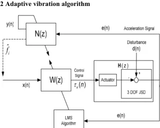
3.2 Adaptive vibration algorithm
ˆ
if
( )z H τ ( )v nˆ
if
ˆ ( )
z
H
( )z H ( ) x n ′( ) x n τ ( )vnFig. 6 Filtered-x least mean square algorithm using ANF The jitter suppression of spacecraft is obtained by the adaptive vibration control algorithm. The vibration controller is the feedforward controller using the adaptive filtered-x least mean square (FLMS) algorithm.[8] In section 3.1, the jitter frequencies are estimated using RLS algorithm. Using this estimated frequency, the reference signal is
1 1 0 ( ) sin(2 ( )) p L k k i n π f n i − = = =
∑
∑
− x )(27)
where p is the number of the notch frequency, L is the filter length.
Using this reference signal, the general least mean square (LMS), FLMS filter is modified as Fig. 5 or Fig. 6 respectively. The FLMS using ANF algorithm is applied to the vibration suppressing experiment without reference sensor.
Then the controller update rule in FLMS using ANF is (n+ =1) ( ) 2 ( )n − µe n ⊗ ( )n
w w H) x
(28)
where ⊗ is the convolution operation and H) is an
(M× vector of filter weight coefficients. At some time n , 1) the vibration control signal ( )τv n is simply a weighted combination of past reference samples
( ) ( ) ( )
v n n n
τ =w ⊗x
(29)
where there are L stages in the filter, w is an (L× vector 1) of filter weight coefficients and x is an (L× vector of 1) reference signal. A block diagram of the adaptive feedforward control arrangement which will be considered in this section is shown in Fig. 24.
The designed controller stability is proved in the following. First, the ANF stability is proved in previous section. The
LMS algorithm converges in mean from (0)w to optimal
weight woif and only if
max
2
0 µ
λ
< <
(30)
where λmax is the largest eigenvalue of the input
autocorrelation matrix. Because computation of λmaxis very
difficult when L is large, the Eq. (30) is replaced with 2 0 x LP µ < <
(31)
where Px≡E x n[ ( )]2 . The filtered-x LMS algorithm will converge within nearly 90deg of phase error between H) and H .[9]
4. EXPERIMENTAL RESULT
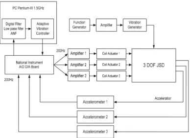
The adaptive vibration control algorithm has been applied to actual experimental demonstration. The overall functional block diagram for the experimental set up is presented in Fig. 7.
The acceleration signal of the each strut is measured by an accelerometer (CXL04LP1, Crossbow) through A/D converter at 200Hz sampling rate. The central processing unit is Pentium-III 1.5GHz processor which computes control signal with digital filter. The controller is commanded by computer output. The computer output signal of the vibration controller is increased by amplifier (BOP 72-3M, KEPCO). In this study, a coil actuator is used to generate the feedback vibration control force required. The coil actuator command is generated at 200Hz. The A/D, and D/A board (PCI-6025E, National Instrument) have 12-bit resolution in discretization. Vibration actuator (VTS-100, Vibration Test System) generates a disturbing vibration in order to simulate spacecraft jitter frequency. The input signal to the vibration generator was generated by function generators or S/W programmed command and the signal is amplified by power amplifier (CE2000, Crown).
Fig. 7 Experimental setup for the jitter suppression Experimental results of 10Hz disturbance are presented in Fig. 8. At initial state, the notch filter frequency is selected as
4Hz. The filter length of w and H) is that L = 200,
M= 200, respectively. The notch filter parameter is set to
0 0.95
ρ = , λ0=0.98 and σ0=0.8 , respectively. The
convergence coefficients are set toµ1=0.0001,µ2=0.00009
and µ3=0.00011, respectively. The control begins at 3sec. After 3sec, the acceleration signal decreased about 9.6dB, 16.5dB, and 7.5dB, respectively. At steady state, the estimated frequency is chattering because the disturbance signal is attenuated. To reduce the chattering of the estimated frequency, the notch filter parameter is changed to ρ =0.98 , λ =0.999 and σ =0.999 at steady state. Figure 9 shows the estimated frequency from the adaptive
0 5 10 15 20 25 30 35 -2 0 2 1 A cc. (m /s 2) 0 5 10 15 20 25 30 35 -2 0 2 2 A cc. (m /s 2) 0 5 10 15 20 25 30 35 -2 0 2 3 A cc. (m /s 2) Time(sec)
Fig. 8 Adaptive vibration control result for 10Hz sine disturbance 0 5 10 15 20 25 30 35 4 6 8 10 12 14 16 Est im at ed d ist u rb an ce f req u en cy( H z) Tim e (se c)
Fig. 9 Estimated jitter frequency for 10Hz sine disturbance
0 5 10 15 20 25 -2 0 2 1 A cc. (m /s 2) 0 5 10 15 20 25 -2 0 2 2 A cc. (m /s 2) 0 5 10 15 20 25 -2 0 2 3 A cc. (m /s 2) Time(sec)
Fig. 10 Adaptive vibration control result for 20Hz sine disturbance 0 5 10 15 20 25 4 6 8 10 12 14 16 18 20 22 E st im at ed d is tur ba nc e fr eque n cy (H z) Tim e (se c)
Fig. 11 Estimated jitter frequency for 20Hz sine disturbance
0 5 10 15 20 25 30 35 40 45 50 -5 0 5 1 A cc.( m /s 2) 0 5 10 15 20 25 30 35 40 45 50 -5 0 5 2 Acc.( m /s 2) 0 5 10 15 20 25 30 35 40 45 50 -5 0 5 3 A cc.( m /s 2) Time(sec)
Fig. 12 Adaptive vibration control result for 10Hz and 20Hz sine disturbance 0 5 10 15 20 25 30 35 40 45 50 4 6 8 10 12 14 16 18 20 22 E st im at ed dis tur ba nc e f re q ue nc y( H z) Time(sec)
Fig. 13 Estimated jitter frequencies for 10Hz and 20Hz sine disturbance 0 5 10 15 20 25 30 35 40 45 50 -4 -2 0 2 Input 1( V o lt ) 0 5 10 15 20 25 30 35 40 45 50 -2 -1 0 1 Input 2( V o lt ) 0 5 10 15 20 25 30 35 40 45 50 -2 0 2 Input 3( V o lt ) Time(sec)
Fig. 14 Control input volts for 10Hz and 20Hz sine disturbance
notch filter.
Experimental results of 20Hz disturbance are presented in Fig. 10. The initial state condition is equal to the 10Hz disturbance case. The notch filter parameter setting is the same as the 10Hz disturbance case. The control begins at 3sec. After 3sec, the acceleration signal decreased about 19.1dB, 10.9dB, and 16.9dB, respectively. To reduce the chattering of the estimated frequency, the notch filter parameter is changed to ρ=0.98 , λ=0.999 and σ =0.999 at steady state. Figure 11 shows the estimated frequency from the adaptive notch filter. The estimated frequency follows well the real disturbance frequency.
Figure 12 shows the experimental results when 10Hz and 20Hz disturbance excite. The initial state condition is equal to the previous case. The notch filter parameter setting is the same as the 10Hz disturbance case. The control begins at 5sec. After 5sec, the acceleration signal decreased about 18.6dB, 23.5dB, and 26.0dB, respectively. To reduce the chattering of the estimated frequency, the notch filter parameter is changed to ρ=0.98 , λ=0.999 and σ =0.999 at steady state. Figure 13 shows the estimated frequency from the adaptive notch filter. The estimated frequencies follow the real disturbance frequency 10Hz and 20Hz. The control input volts are shown in Fig. 14.
It is consider the following rule to select the convergence coefficient µ . Since the upper bound on µ is inversely
proportional to L in Eq. (31), small µ is used for
large-order filters. Since µ is made inversely proportional to the input signal power, weaker signals can use a larger µ and stronger signals have to use a smaller µ.
Instead using constant ρ ,λ and σ , the notch filter parameter increases, respectively. These parameters, as mentioned already, are so important to determine the disturbance frequencies. If the forgetting factor λ is so small, the estimation performance is degraded. But if it is too large, the performance is also degraded for the case of time varying parameter estimation. In the experimental investigation, the selection of an appropriate forgetting factor is important for the resulting performance of the vibration controller.
5. CONCLUSION
In the present study, the jitter isolation of spacecraft has been examined. In space there could be many disturbance sources such as solar radiation pressure, and aerodynamic forces which inhibit high accuracy. The main source of spacecraft vibration is the RW or CMG. The disturbances are in the high frequency domain above 10Hz and they degrade spacecraft pointing performance and communication accuracy to the ground station. To attenuate the disturbance of the spacecraft, FLMS using ANF was applied to the jitter suppression device. Adaptive notch filter (ANF) finds the disturbance frequency and the reference signal in FLMS is generated by this notch frequency. The design parameters of the notch filter are updated continuously using recursive least square (RLS) algorithm. Therefore, the adaptive FLMS algorithm is applied to the vibration suppressing experiment without reference sensor. Significant reductions of vibration level have been observed for real-time adaptive controls. The designed FLMS using ANF has a good performance without the reference.
ACKNOWLEDGMENTS
The present work was supported by National Research Lab. (NRL) Program (M1-0203-00-0006) by the Ministry of Science and Technology, Korea. Authors fully appreciate the financial support.
REFERENCES
[1] S. J. Elliott, I. M. Stothers, and P. A. Nelson, “A multiple error LMS algorithm and its application to the active control of sound and vibration,” IEEE Trans. of ASSP, Vol. 35, pp. 1423-1434, 1987.
[2] L. J. Eriksson, M. C. Allie, and R. A. Greiner, “The selection and application of IIR adaptive filters for use in active sound attenuation,” IEEE Trans. of ASSP, Vol. 35, pp. 433-437, 1987.
[3] W. T. Baumann, and H. H. Robertshaw, “Active structural ascoustic control of broadband disturbances,”
Journal of the Acoustical Society of America, Vol. 88,
pp. 3202-3208, 1992.
[4] B. Widrow, and S. D. Stearns, Adaptive Signal
Processing, Prentice Hall, New Jersey, 1985.
[5] D.V. Rao, and S.Y. Kung, “Adaptive Notch Filtering for the Retrieval of Sinusoids in Noise,” IEEE Trans. On
Acoustic, Speech, Signal Processing, Vol. 32, pp.
791-802, 1984.
[6] P. A. Regalia, “An Improved Lattice-Based Adaptive IIR Notch Filter,” IEEE Trans. on Acoustic Speech,
Signal Processing, Vol. 39, pp. 2124-2128, 1991.
[7] S. Haykin, Adaptive Filter Theory, 4th ed., Prentice
Hall, New Jersey, 2002, Chaps. 9
[8] C. H. Hansen, and S. D. Snyder, Active Control of Noise
and Vibration, E & FN Spon, London, 1997.
[9] S. M. Kuo, and D. R. Morgan, Active Noise control