Walk Simulations of a Biped Robot

1. INTRODUCTION

Fig.1 Skeleton diagram of the robot

Walk Simulations of a Biped Robot

S.Lim*, K.I.Kim

**

_{, Y.I.Son}

**

_{, and H.I.Kang}

***

* Department of Mechanical Engineering, Myongji University, Yongin, Korea (Tel : +82-31-330-6428; E-mail: [email protected])

**Department of Electric Engineering, , Myongji University, Yongin, Korea (Tel : +82-31-330-6356/6358; E-mail: kkl/[email protected])

***Department of Information Engineering, , Myongji University, Yongin, Korea (Tel : +82-31-330-6757; E-mail: [email protected])

Abstract: This paper is concerned with computer simulations of a biped robot walking in dynamic gaits. To this end, a three-dimensional robot is considered possessing a torso and two identical legs of a kinematically ingenious design. Specific walking patterns are off-line generated meeting stability based on the ZMP condition. Subsequently, to verify whether the robot can walk as planned, a multi-body dynamics CAE code has been applied to the corresponding joint motions determined by inverse kinematics. In this manner, complex mass effects could be accurately evaluated for the robot model. As a result, key parameters to successful gaits are identified including inherent characteristics as well. Also, joint actuator capacities are found required to carry out those gaits.

Keywords: Walking Pattern Generation, Inverse Kinematics, Dynamic Stability, ZMP, Actuator Specification, Humanoid

Lately, biped robots are attracting extraordinary attention because of its potential to coordinate with people in the human-friendly environment. The way they walk is generally classified into two categories: static and dynamic gaits [1,2]. Whereas the static gait is conceptually so simple as to be widely implemented at present [2], the dynamic gait is rather difficult in terms of securing stability due to inertia forces. This is why only a few humanoids have been reported successful so far [3-5].

This motivates us to pursue a methodology to find proper dynamic gait patterns and actuator capacities prior to actual robot construction. To this end, a 3-D biped robot in the companion work [6] is reconsidered, a set of inverse kinematic solutions is derived, and details are established as to how walking patterns can be generated meeting stability based on the ZMP condition. Finally a multi-body dynamics CAE code, namely ADAMS [7], is utilized in order to verify whether the robot can walk as planned in the presence of mass and ground effects.

general. To deal with such a problem, coordinate frames are defined as in Fig. 2: Cartesian inertial coordinate frame {0} with X -axis pointing forward, and link-fixed coordinates frames, {1} through {4}, with

x

-axes initially coincident with X and z-axes aligned along individual links. Then, for example, the relative position of the right foot to the torso,

(= ), is expressed as below in terms of {1}. u

rf /

r rrf −ru Upon simulations, a dynamic gait of average speed 86

mm/s, comparable to existing humanoids converted to the proposed biped’s size, was confirmed successful. The overall postures and torso motions during that locomotion are presented. Also, joint actuator capacities are found required to carry out the gait involving angular displacements, torques, and powers. As a result, key parameters to successful dynamic gaits and their inherent characteristics in contrast to static ones could be identified. They matter particularly in the light of larger-scale robots to be built.

rf rs rt u u rf

x

R

x

R

x

R

x

r

/ 1 21 2 31 3 41 4 1

₌

₊

₊

₊

_{, (1)} where ,1 , , , and . T u rf/ [x y z] 1_{r =} T sz sy sx l l l ] T u

=

[

a

1

a

2

a

3

]

x

fz fy fx rf l[ l l 4_{x =} T tz ty tx rt [l l l ] 2_{x =} T rs [ 3_{x = ]}

2. INVERSE KINEMATICS

The biped robot under present investigation has a torso and duplicate legs as in Fig.1. Each leg has 6 degrees of freedom (DOFs), first three of them orthogonally intersecting at the pelvis joint, next one at the knee, and the last two at the ankle. Those rotational axes are arranged in sequence of yaw (M1/M7), roll (M2/M8), pitch (M3/M9), pitch (M4/M10), pitch (M5/M11), and roll (M6/M12) from the top.

Actually, except for , , , , and

respectively standing for torso sizes, thigh length, shin length, longitudinal and vertical distances of the foot’s centroid from the origin of {4}, the other dimensions are all zeros. Meanwhile, the involved rotation matrices between the frames are as follows with abbreviations such as

) 3 , 2 , 1 (

i

=

a

_i

l

_tz

l

_sz l_fx i

s

fz l i

ϑ

sin

=

, i i

c

=

cos

ϑ

,

s

_ij

=

sin(

ϑ

_i

+

θ

_j

)

, and

c

_ij

=

cos(

ϑ

_i

+

θ

_j

)

: Although humanoid robots consist of numerous DOFs, each

Fig.2 Coordinate frames for kinematics

          − + − + + − + − = 3 2 2 3 2 3 1 3 2 1 2 1 3 1 3 2 1 3 1 3 2 1 2 1 3 1 3 2 1 1 2 c c s s c s s c s c c c c s s s c s c c s s c s c c s s s R ,           − + − + + − + − = 34 2 2 34 2 34 1 34 2 1 2 1 34 1 34 2 1 34 1 34 2 1 2 1 34 1 34 2 1 1 3 c c s s c s s c s c c c c s s s c s c c s s c s c c s s s R , . 6 2 345 6 2 6 2 1 345 6 1 345 6 2 1 6 2 1 345 6 1 345 6 2 1 6 2 345 2 6 345 2 6 2 1 345 6 1 345 6 2 1 345 1 345 2 1 6 2 1 345 1 6 345 6 2 1 345 1 345 2 1 1 4      − − + − + +      + − + + − + − + + − = s s c c c s c c s c s c c s c s c s s c c c s s s c s c c s s c c c c s s s c s s c c s s s c c c s s c s c s s s c c s s s R

It turns out that the successive three rotations along the pitch direction can be treated as an angle, making kinematics easier to handle. Hence, given arbitrary positions and null orientations (i.e., ) between the torso and the foot, a set of inverse kinematics solutions is analytically derived when walking is made along a straight line:

I R= 1 4 0 1=

θ

,

θ

₂

=

ATAN

2

(

s

₂

,

c

₂

)

,

θ

₃

=

2

ATAN

(

u

)

,

)

,

(

2

4 4 4

=

ATAN

s

c

θ

,

θ

₅ =−

θ

₃−

θ

₄ ,

θ

₆ =−

θ

₂ , (2a,b,c,d,e,f)

If the forcing term, ZMP coordinate, is given as a continuous time function of first or higher order, either the foot size should be excessively large or the stride length should be small for robots to be stable during single-support phase (SSP). To avoid such shortcomings, it is desirable to let ZMP positions piecewise constant. Then, above two ODEs can be solved independently of each other to obtain hyperbolic torso motions for generic initial conditions such as

0

)

0

(

x

x

b = ,

x

&b

(

0

)

=

x

&0,

y

b

(

0

)

=

y

0, and

y

&b

(

0

)

=

y

&0.

where 34 3 2 2 ) ( c l c l a y s sz tz + − − = , c₂ =± 1 s− ₂2 , , ) ( } ) {( ) ( ) ( 4 1 2 4 2 2 1 2 4 4 s l l a x s l l a x c l l c l l u sz fx sz fx sz tz sz tz + − − − − − − + ± + = 2 4 4 1 c s =± − , . 2 ) ( ) ( ) ( 2 2 2 3 2 2 2 1 4 tz sz tz sz fz fx l l l l l a z a y l a x c = − − + − + − − − −

3. WALKING PATTERN GENERATION

Just like humans, robots will determine the body trajectory after landing positions of feet are first assigned. However, its

associated procedures can be more or less different depending on gait forms. In the case of dynamic gaits, the upper body must move so that the ZMP position in Eq. (3) always lies in the stable region formed as a convex hull connecting all contact points. ) ( ) ( 1 1 1 1 g z m I z x m x g z m x i n i i n i n i iy iy i i i i i n i i ZMP + − − + =

∑

∑

∑

∑

= = = = && & && && Ω (3a) ) ( ) ( 1 1 1 1 g z m I z y m y g z m y i n i i n i n i ix ix i i i i i n i i ZMP + − − + =

∑

∑

∑

∑

= = = = && & && && Ω (3b)

Once motions of the feet and the torso are set up in the Cartesian coordinate, corresponding joint motions are obtained via the inverse kinematics in Eq. (2), and actually carried out by joint controllers at a lower hierarchical level.

Until now, based on the pattern-generation timing off- [3,5] and on-line [8] methods have been proposed. However, the former is more feasible in view of practical constraints. In this context, adopting the hyperbolic patterns [3] that belong to the off-line approach, its undisclosed derivation process is detailed first. Subsequently the scheme is extended to the initial state characterized by the stationary stance with feet apart sideways.

3 .1 Hyperbolic walking pattern (steady state)

The ZMP equation (3) is quite complicated and hard to apply as it is. So, some simplification is made taking into account that robots tend to have more massive torso than limbs and maintain same height while walking. Then Eq. (3) reduces to non-homogeneous, 2nd order ODEs with constant coefficients: ZMP b b a x a x x_{&& −} 2 ₌₋ 2 _{, , (4a,b)} ZMP b b a y a y y_{&& −} 2 ₌₋ 2

where subscript

b

indicates the upper body, and b

z

g

a

=

/

is a positive constant. ZMP ZMP b

_a

at

x

x

at

x

x

x

=

(

−

)

cosh

+ 0

sinh

+ 0 & (5a) ZMP ZMP b

y

y

at

y

_a

at

y

y

=

(

−

)

cosh

+ 0

sinh

+ 0 & (5b)

To prevent Eq. (5) from monotonically growing, the first two coefficients on each right hand side should be tuned opposite in signs. This can be possible by moving the torso at

a constant speed during double-support phase (DSP), and variable speed during SSP alone with ZMP values greater than initial positions. Figure 3 illustrates such a walking pattern, in which , , and denote respectively negative, zero, and positive acceleration time intervals during SSP along x-axis, and the constant–speed time interval during DSP along both x- and y-axes.

1

t

t

₂ 4

t

3

t

Likewise, for interval III (

0

≤

τ

≤

t

₃)

2

sinh

)

(

xS _ZMP b

_a

a

x

v

x

τ

=

τ

+

, (9a)

x

t

x

_b

(

₃

)

=

′

,

x

&_b

(

t

₃

)

=

v

_xD. (9b,c) The same reasoning leads to Eq. (10) for the entire SSP interval (

0

≤

τ

≤

t

₅), which describes the lateral motion. As far as the lateral motion is concerned, robots will only

decelerate throughout SSP that lasts for

t

₅(=

t

₁+

t

₂+

t

₃

s

x

). Moreover, and mean respectively the ZMP positions during intervals I and III along x-axis, the steady stride length, and finally the torso position at the end of SSP. 1 ZMP

x

x

_ZMP2

x′

ZMP y ZMP b

_a

a

y

v

a

y

y

y

(

τ

)

=

(

₀

−

)

cosh

τ

+

sinh

τ

+

, (10a)

0 5

)

(

t

y

y

_b

=

,

y

&_b(

t

₅)

=

−

v

_y. (10b,c) Hence, inputting gait parameters such as desired ZMP

values ( , , ), walking speed ( ), and

others ( , , ), Eqs. (6)~(10) can be solved for the following unknowns: 1 ZMP

x

a

x

₀ 2 ZMP

x

s

x

ZMP

y

v

_xD ) ( ) ( ln 2 1 1 0 1 0 1 ZMP xD ZMP xD

x

x

a

v

x

x

a

v

a

t

−

+

−

−

=

, (11a) 1 1 1 0 )sinh cosh (

x

x

at

v

at

a

v

_xS

=

−

_ZMP

+

_xD , (11b) 0 2 1

x

x

x

x

′

=

_ZMP

+

_ZMP

−

, (11c) xD s

v

x

x

x

a

t

=

( 0

+

/2)

−

′

4 , (11d) ) 1 ( 2 ) 1 ( ) 1 ( 4 4 0

at

_q

y

_at

q

_q

y

ZMP

+

−

−

−

=

, (11e) 4 0 2

t

y

v

_y

=

, ) ( ) ( ln 1 0 0 5 ZMP y ZMP y y y a v y y a v a t − + − + − = , (11f,g) xS ZMP ZMP v x x t 2 1 2 − = , (11h)

Fig.3 Hyperbolic walking pattern

Since the traveled distances during intervals I and III are designed equal, where . ) ( ) ( } ) ( }{ ) ( exp{ 1 0 1 0 0 1 1 2 ZMP xD ZMP xD xS xD ZMP xS ZMP ZMP x x a v x x a v v v x x a v x x a q − + − − ⋅ + − − = 0 1 2

x

x

x

x

′

−

ZMP

=

ZMP

−

. (6) In addition, Eq. (7) holds for the constant speeds while and respectively mean their magnitudes for SSP and DSP commonly along x-axis, and

v

that for DSP along y-axis.

xS

v

xD

v

y Remarkably, for Eq. (10a) to be valid, one condition of

) (x ₁ x₀ a

v_xD > _ZMP − should be met, which requires that the average speed during SSP be slower than the constant speed during DSP unless robots are taller than 9.8 m.

2 1 2

t

x

x

v

ZMP ZMP xS

−

=

, 4 0

/

2

)

(

t

x

x

x

v

s xD

′

−

+

=

, (7a,b) _{As they are, however, aforementioned motions are not}

applicable to the initial stationary posture with two supporting feet apart sideways. Therefore, the pattern generation procedure needs extension to the transient state without causing infinite accelerations.

4 0

2

t

y

v

y

=

(7c)

Accordingly, for interval I (

0

≤

τ

≤

t

₁) the body position equals to Eq. (8a) with terminal conditions in Eqs. (8b) and (8c) resulting from continuity of positions and velocities.

3 .2 Hyperbolic walking pattern (transient state)

First of all, it is necessary to shift the torso either right or left assigning ZMP a nonzero constant coordinate, e.g.,

( ). Then, the body motion can be obtained

from Eq. (5a) with due consideration of zero initial conditions: D ZMP D ZMP y x ₀ , ₀ 1 1 0

)

cosh

sinh

(

)

(

xD _ZMP ZMP b

x

x

a

v

_a

a

x

x

τ

=

−

τ

+

τ

+

, (8a) 1 1

)

(

_ZMP b

t

x

x

=

,

x

&_b

(

t

₁

)

=

v

_xS. (8b,c) D ZMP D ZMP b t x at x x ()=− ₀ cosh + ₀ for 0≤t≤t* (12)

As the DSP ends, let the leg farther from the torso leave the ground and swing forward by commanding another

constant ZMP at ( ). During such SSP

( ), the body trajectory can be found as in Eq. (13) if motional continuity up to velocities is imposed across the two successive phases.

2 / s x S ZMP0 S ZMP y x ₀ , * 0≤

τ

≤

τ

, cosh ) cosh ( sinh ) sinh ( ) ( 0 0 0 * 0 * 0 S ZMP S ZMP D ZMP D ZMP D ZMP b x a x x at x a at x x + − + − + − =

τ

τ

τ

τ

τ

τ

a x x at x a a at ax x S ZMP D ZMP D ZMP D ZMP b sinh ) cosh ( cosh ) sinh ( ) ( 0 0 * 0 * 0 − + − + − = & (13a,b) Application of the same motional continuity gives Eq. (14) between the transient SSP and the beginning of steady DSP.

s

b x

x (

τ

*)= , x&_b(

τ

*)=x&_s (14a,b) In fact, the foregoing equation involves four unknowns. So, designating as inputs two of them, namely t and , the others can be uniquely solved for:

*

_τ

* } sinh ) ( sinh sinh { ) cosh 1 ( sinh * * * * * * 0

_τ

_τ

τ

τ

a t a at a a x a ax x s s D ZMP − + + − − − − = & , } sinh ) ( sinh sinh { )} ( cosh {cosh )} ( sinh {sinh * * * * * * * * * * 0 τ τ τ τ τ τ a t a at a t a a x t a a ax x s s S ZMP _{− + + −} + − + + − − = & (15a,b) It is obvious that from the same principle, ZMP positions along the lateral direction can be readily obtained which replace

x

s by s in Eq. (15). Inherent to the solution procedure, it is left to check whether the such-calculated ZMP positions lie in the stable region before proceeding.

y

4. DYNAMIC SIMULATION

The designed biped robot is 478mm tall and as heavy as 2.24kg, of which about 80% is the torso’s weight. Refer to Table 1.

Table 1 Specifications of the robot

Part Size [mm] Mass [kg]

Body 196(W)x150(H)x60(T) 1.781

Right Leg 325(L) 2.150e-1

Left Leg 325(L) 2.150e-1

Right Foot 50(W)x110(L)x3(T) 1.546e-2 Left Foot 50(W)x110(L)x3(T) 1.546e-2

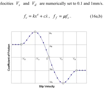
Total - 2.242 The normal reaction force arising from the ground contact is modeled as sum of nonlinear spring and viscous damping forces as in Eq. (16a), where

x

and represent respectively the penetration depth and its rate; =10

x&

k 2_N/mm; =1.5; =10Ns/mm. Along with it, the friction force that is the ultimate source of thrust is regarded to take place in form of Coulomb friction, i.e., Eq. (16b). The friction coefficient

e

c

µ

takes either

µ

_s(=0.8) or

µ

_d(=0.7) depending on slip velocity. Figure 4 shows the details, where transition

velocities V_s and V_d are numerically set to 0.1 and 1mm/s.

kxe / s x y_ZMP x c fc = + &, ff =

µ

fc. (16a,b) Fig.4 Friction coefficient vs. slip velocity

As an example, a set of input gait parameters is assumed:

=395mm, =0mm, =100mm, = ,

= , =68mm, =100mm/s, =0.2s,

=0.3s. In return, Eq. (11) computes = =0.1464s, =0.1597s, =0.1250s, =0.4526s so that the steady walking period =1.152s. For the total simulation time of 1.75s including three steps counted from the stationary state, the position and velocity of the body evolve as in Figs. 5 and 6. b z ZMP x *

τ

2 t 0 x 4 t s T s x 5 t 1 ZMP x 1 t

t

3 8 / s x * t 2 4 vxD

Fig.5 Body positions including the initial transient

Next figures exhibit dynamic simulation results obtained by use of ADAMS. Displayed in Fig. 10 are the snapshots of animated walking motion captured at an equal interval: Initially both legs are intended to bend (M3=M9=22o_, M4=M10=-39.53o_{, M5=M11=17.53}o_{). However, such initial} conditions happened to place the both feet slightly above the ground. Eventually it made the robot fall down later on till 0.05s due to gravity, and caused unusually large torques at the touch down moment in Fig. 13, which readers are advised to ignore. Figure 11 shows the torso motions during associated, perfect walk with no bouncing from the ground. Resulting motions prove smooth due to continuous positions and velocities.

Besides, both ZMP positions of the transient walk turn out well inside the stable region, being (-19.3276, -32.4849) and (25.9193, 80.3014) [mm] respectively as plotted in Fig. 7. In so doing, the foot trajectories originally drafted as in Figs. 8 and 9 were smoothed out by a quintic function in Eq. (17).

         ≤ ≤ ≤ + − − + − − − − − ≤ = 2 2 2 1 1 3 1 3 1 2 4 1 4 1 2 5 1 5 1 2 1 1 for for ) ( ) ( 10 ) ( ) ( 15 ) ( ) ( 6 for ) (

τ

τ

τ

τ

τ

τ

τ

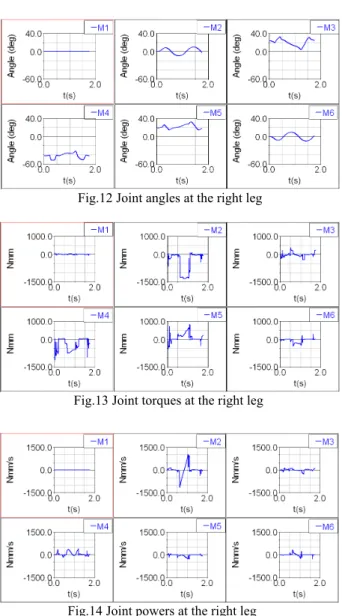
t A t A t h A A t h A A t h A A t A t f ,(17)

From Figs. 12~14, the joint actuator capacities regarding angles, torques, and powers can be specified at the right leg during the gait. In the case of torques, a similar trend but much smaller in magnitude appears compared to static gaits [6]. Yet, larger powers are seen necessary for dynamic gaits due to faster walking speed.

where

A₁

and

A₂

are step magnitudes,

τ and

₁

τ

₂

the initial and the final instants of the transition period

of duration . Such a measure is justified by that

otherwise abrupt motions are unrealizable in practice.

h

Based on the simulation results, the characteristics of dynamic gaits can be summarized as in Table 2. A dynamic gait of average speed 86 mm/s is achieved. Such a speed is comparable to existing humanoids converted to the proposed biped’s height: The corresponding performances of the present one, KHR-1 [5], Johnnie [3], Asimo are respectively 0.18s-1_, (22cm/s)/(120cm)=0.18s-1_{, (33cm/s)/(180cm)=0.18s}-1_{, and} (44cm/s)/(120cm)= 0.36s-1_.

Fig.7 Position trajectory (XY plot)

Fig.8 Foot motions along X-direction

0s 0.35s 0.70s

1.05s 1.40s 1.75s

Fig.10 Snapshots of the dynamic gait

Fig.12 Joint angles at the right leg

Fig.13 Joint torques at the right leg

Fig.14 Joint powers at the right leg

Referring to the mass effect on walking speed, any constant speed can be maintained regardless of robot mass as implied also by Eq. (5). This is contrary to static gaits. Not to mention that the heavier robots weigh, more torque and power are required in proportion.

Table 2 Characteristics of dynamic gaits

average speed 86 [mm/s]

maximum required torque and the corresponding axis

Abt. 1300 [Nmm] at M2/M8 maximum required power and the

corresponding axis Abt. 1 [W] at M2/M8 walking speed negligible required torque linear mass effects on

required power linear

gear reduction less favorable

5. CONCLUSIONS

In this paper, a biped robot is proposed along its inverse

kinematics solution, and a hyperbolic form of dynamic walking pattern is presented applicable even to the transient state of biped robots. Such a pattern was proved via dynamic simulations on a flat surface. As a result, we could find primary parameters such as walking period and actuator capacities for successful locomotion, and major characteristics of dynamic gaits as well.

As opposed to static ones, dynamic gaits do not degrade in speed as mass grows, requiring far less torques. Instead of torque, power is more critical for dynamic gaits to maintain a speed regardless of mass. Hence, for larger-scale robots it is desirable to adopt dynamic gaits by employing actuators of sufficient power and moderate gear reductions.

ACKNOWLEDGMENTS

This work was supported by Korea Science and Engineering Foundation Grant (KOSEF-R-01-2003-000-10014-0). Authors would like to deeply acknowledge the support.

REFERENCES

[1] M.Vukobratovic, B.Borovac, D.Surla, and D.Stokic,

Scientific Fundamentals of Robotics 7: Biped Locomotion, Springer-Verlag, 1990.

[2] S.N.Oh, K.I.Kim, and S.Lim, “Motion control of biped robots using a single-chip drive,” IEEE Int. Conf. on

Robotics and Automation, 2003.

[3] K.Loffler, M.Gienger, and F.Pfeiffer, “Sensor and control design of a dynamically stable biped robot,” IEEE Int.

Conf. on Robotics and Automation, 2003.

[4] J.J.Kuffner,Jr., S.Kagami, K.Nishiwaki, M.Inaba, and H.Inoue, “Dynamically-stable motion planning for humanoid robots,” Autonomous Robots, Vol. 12, pp.105-118, 2002.

[5] J.H.Kim, S.W.Park, I.W.Park, and J.H.Oh, “Development of a humanoid biped walking robot platform KHR-1 - initial design and its performance evaluation,” The 3rd

IARP Int. Workshop on Humanoid and Human Friendly Robotics, 2002.

[6] S.Lim and I.Ko, “Gait simulations of a biped robot: (I) static gaits,” Spring Conf. of KSME, 2005. (in Korean) [7] Mechanical Dynamics Inc., Basic ADAMS Full

Simulation Training Guide, 2001.

[8] T.Sugihara, Y.Nakamura, and H.Inoue, “Realtime humanoid motion generation through ZMP manipulation based on inverted pendulum control,” IEEE Int. Conf. on

Robotics and Automation, 2002.