Autonomous Coil Alignment System Using Fuzzy Steering Control for Electric Vehicles with Dynamic Wireless Charging

(1)

Research Article

Autonomous Coil Alignment System Using Fuzzy Steering

Control for Electric Vehicles with Dynamic Wireless Charging

Karam Hwang,

1

Jaehyoung Park,

1

Dongwook Kim,

1

Hyun Ho Park,

2

Jong Hwa Kwon,

3

Sang Il Kwak,

3

and Seungyoung Ahn

1

1_{Korea Advanced Institute of Science and Technology (KAIST), Daejeon 34141, Republic of Korea} 2_{The University of Suwon, Hwasung 445-743, Republic of Korea}

3_{Electronics and Telecommunications Research Institute (ETRI), Daejeon 34129, Republic of Korea}

Correspondence should be addressed to Seungyoung Ahn; [email protected] Received 4 September 2015; Accepted 18 November 2015

Academic Editor: Shengbo Eben Li

Copyright © 2015 Karam Hwang et al. This is an open access article distributed under the Creative Commons Attribution License, which permits unrestricted use, distribution, and reproduction in any medium, provided the original work is properly cited. An autonomous coil alignment system (ACAS) using fuzzy steering control is proposed for vehicles with dynamic wireless charging. The misalignment between the power receiver coil and power transmitter coil is determined based on the voltage difference between two coils installed on the front-left/front-right of the power receiver coil and is corrected through autonomous steering using fuzzy control. The fuzzy control is chosen over other control methods for implementation in ACAS due to the nonlinear characteristic between voltage difference and lateral misalignment distance, as well as the imprecise and constantly varying voltage readings from sensors. The operational validity and feasibility of the ACAS are verified through simulation, where the vehicle equipped with ACAS is able to align with the power transmitter in the road majority of the time during operation, which also implies achieving better wireless power delivery.

1. Introduction

It is notable that commercialization of electric vehicles (EVs) is becoming more widespread around the world in order to reduce the serious issues related to global warming and energy depletion that are being faced today. However, the EV poses some major flaws which are its high cost and long charging times, which inevitably directs consumers to still resort towards conventional internal combustion engine (ICE) vehicles. Those major flaws are mainly caused due to the drawbacks of current battery technology. To minimize the drawbacks caused from batteries, EVs with dynamic wireless charging systems have been developed. Dynamic wireless charging system allows the vehicle to charge in real time while in motion, which also allows the reduction of the overall battery capacity in the vehicle. This provides the benefit of reducing overall vehicle cost and reduced charging times. Dynamic wireless charging systems are a part

of wireless power transfer (WPT) technology, where power can be transferred from one circuit to another circuit without any physical contact or wiring. WPT technologies are being studied widely around the world as an anticipation to reduce or eliminate any physical wiring elements that restrict power supply to electric or electronic devices [1]. WPT technology has been introduced by N. Tesla in 1914, but it is not until recently that WPT technology has been applied into com-mercial electronic devices, biomedical products, industrial applications [1–4], and now stationary and dynamic wireless charging vehicles.

A WPT system consists of the power transmitter portion and power receiver portion. The power transmitter portion is composed of a power source and coil, where the power source is generated into an electromagnetic field as it enters through the coil. The power receiver portion, which consists of another coil, will convert the received electromagnetic field into usable energy that can power another source [5–7].

(2)

For every WPT system, there is a specific alignment range between the power transmitter and power receiver in which maximum power can be transferred, and this alignment range will vary by system due to its intrinsic parameters such as resistance, inductance, and capacitance [2]. When the range goes past the specific alignment, the power transfer capacity will drop or become near zero in certain cases [7].

In the case of dynamic wireless charging systems for road vehicles, keeping the alignment range becomes more difficult since the vehicle’s lateral displacement will continuously change during motion. To achieve maximum power, the driver will have to pay careful attention in keeping the power receiver on the vehicle aligned with the power transmitter, which is installed beneath the center of each road lane. Even when it is assumed that the driver kept the vehicle aligned with the center of the road lane, it does not guarantee that the vehicle’s receiver is in perfect alignment with the power transmitter, since the power transmitter is not visible (as it is installed beneath the road). In addition, keeping the vehicle aligned at the center of the road will require a lot of concentration, which can distract the driver to oncoming dangers and can lead to potential car accidents.

To resolve such misalignment issues in dynamic wireless charging systems, many researches have been conducted to increase their alignment range through efficient power receiving modules [6, 8–10]. However, in certain cases, these methods may become difficult or very costly to implement [2]. Therefore in this paper, an autonomous coil alignment system (ACAS) is proposed, which can be implemented for generally all vehicles equipped with dynamic wireless charging systems. The proposed system will detect the mis-alignment between the power receiver and power transmitter through sensors. When misalignment is detected, the vehicle will adjust itself through autonomous steering control in order to correct the alignment between the vehicle’s power receiver and the power transmitter. Through this system, the vehicle will be able to achieve maximum power delivery with minimum driver effort. In addition, since the ACAS operates in a similar manner with the lane keeping assist system (LKAS), the ACAS will be able to keep the vehicle along the center of the road lane, thus providing more safety for the driver as well.

The paper will first describe the principles of WPT and the background research on dynamic wireless charging of vehicles. Then the motivation of the proposed ACAS and its technical operation concept is described, followed by simulation settings and tests to verify its feasibil-ity.

2. Principles of the Wireless Power Transfer

(WPT) System

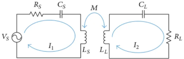
The fundamental circuit of the wireless power transfer system is described as shown in Figure 1. The system is comprised of two RLC circuits: the circuit on the left-side is the source coil circuit (power transmitter) and the circuit on the right side is the load coil circuit (power receiver).

VS RS CS CL I1 _L S LL RL I2 M

Figure 1: Circuit schematic of the source circuit and load circuit in wireless power transfer (WPT).

The equation for source coil and the load coil based on Figure 1 is expressed as (𝑅_𝑆+ 1 𝑗𝜔𝐶_𝑆 + 𝑗𝜔𝐿𝑆) 𝐼1− 𝑗𝜔𝑀𝐼2− 𝑉𝑆= 0, (𝑅_𝐿+ 1 𝑗𝜔𝐶𝐿 + 𝑗𝜔𝐿𝐿) 𝐼2− 𝑗𝜔𝑀𝐼1= 0. (1)

In (1), each of 𝑅_𝑥, 𝐶_𝑥, and 𝐿_𝑥 represents the resistor,

capacitor, and inductor component, while𝑆 or 𝐿 subscript of

a certain component represents the source coil or load coil,

respectively.𝜔 represents the frequency, and 𝐼₁,𝐼₂represent

the current flowing in the source coil and the load coil, respectively, which are expressed as follows:

𝐼1=𝑅𝐿+ 1/𝑗𝜔𝐶_𝑗𝜔𝑀𝐿+ 𝑗𝜔𝐿𝐿𝐼2,

𝐼2=_(𝑅 𝑗𝜔𝑀

𝑆+ 1/𝑗𝜔𝐶𝑆+ 𝑗𝜔𝐿𝑆) (𝑅𝐿+ 1/𝑗𝜔𝐶𝐿+ 𝑗𝜔𝐿𝐿) + 𝜔2𝑀2

⋅ 𝑉𝑆.

(2)

𝑀 shown in (1) to (2) is the mutual inductance that occurs between the source coil and load coil while operating in resonant frequency. This is expressed as

𝑀 = 𝑘√𝐿_𝑆𝐿_𝐿. (3)

In (3),𝑘 is a value ranging between 0 and 1 and represents the

coupling coefficient between the source coil and the load coil. When the value is near 1, it implies that the coupling between the source coil and load coil is very strong and will result in higher mutual inductance. When the value is near 0, it implies that the coupling between the source coil and load coil is very weak and will result in a lower to near nonexistent mutual

inductance. In WPT, a larger𝑀 value usually facilitates more

effective power transfer [11]. Based on (2), the power from the source coil can be determined as follows:

𝑃𝑆= 𝐼1𝑉𝑆 = 𝑅𝐿+ 1/𝑗𝜔𝐶𝐿+ 𝑗𝜔𝐿𝐿 (𝑅𝑆+ 1/𝑗𝜔𝐶𝑆+ 𝑗𝜔𝐿𝑆) (𝑅𝐿+ 1/𝑗𝜔𝐶𝐿+ 𝑗𝜔𝐿𝐿) + 𝜔2𝑀2 ⋅ 𝑉2 𝑆. (4)

(3)

Inverter Rectifier Motor Battery Regulator Attracted magnetic flux Magnetic core Pick-up coil Road Vehicle

Embedded power line segments Power line

segment (off) segment (off)Power line segment (on)Power line segment (off)Power line

Figure 2: Block diagram of the OLEV system.

Similarly, using (2), the power from the load coil can be determined as 𝑃𝐿= 𝐼22𝑅𝐿 =󵄨󵄨󵄨󵄨󵄨󵄨󵄨󵄨 󵄨󵄨 −𝜔2_𝑀2 {(𝑅𝑆+ 1/𝑗𝜔𝐶𝑆+ 𝑗𝜔𝐿𝑆) (𝑅𝐿+ 1/𝑗𝜔𝐶𝐿+ 𝑗𝜔𝐿𝐿) + 𝜔2𝑀2}2 󵄨󵄨󵄨󵄨 󵄨󵄨󵄨󵄨 󵄨󵄨 ⋅ 𝑉𝑆2𝑅𝐿. (5)

The equations shown from (1) to (5) are the general principle guidelines used to design a WPT system including vehicles with dynamic wireless charging systems, and the final gener-ated power shown in (5) will power the components in the power receiving portion.

3. Concept on Electric Vehicles (EVs) with

Dynamic Wireless Charging

The development on EVs using dynamic wireless charging has been progressing on for the past few decades, and some of the recent advancements (and commercialization) have been made such as the online electric vehicle (OLEV) [11–15]. It has been widely recognized and commercialization of these vehicles is currently progressing in Korea [13]. Figure 2 shows the basic principle of the EV’s dynamic wireless charging system (OLEV).

The power transmitter part of the system consists of the inverter and power line, where the inverter provides power to the power lines that are installed beneath the road. The power line is installed as power line segments, where the inverter will only turn on the segment where the vehicle is located in order to mitigate the inefficiency of the power supply [14]. The inverter receives 60 Hz power from the main electrical power plant and converts into a specific constant current at specific resonant frequency. In OLEV systems, the constant current ranges between 200 A to 260 A, and the resonant frequency is set at 20 kHz [11].

The power receiving part of the system is attached on the bottom of the vehicle chassis, which consists of the pick-up coil, magnetic core, rectifier, and regulator. The magnetic core of the receiving system captures the magnetic flux from the power lines and will induce voltage along the power lines. The induced voltage is converted into DC voltage through

Pick-up coil

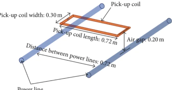
Power line Pick-up coil width:0.30 m

Air gap:0.20 m Pick-up co il length: 0.72m Distance b_{etween p} ower lines: 0.72m

Figure 3: The model and parameters of the pick-up coil and power line used in the Maxwell simulation.

the rectifier and then converted into the desired voltage range through the regulator. A small portion of the received power is used to drive the motor while the rest is used to charge the battery when the vehicle is in motion. When the vehicle is not in motion, all the received power is used to charge the battery. The power receiving part is installed as modules, where each power receiving module is capable of generating 20 kW of power. In case of the OLEV bus, five modules were installed in order to achieve a total of 100 kW target power [11].

4. Motivation for the Coil Alignment

System (ACAS)

As mentioned earlier about EVs with dynamic wireless charg-ing, lateral misalignment between the power transmitter and the power receiver will inevitably occur, which will result in reduced power transfer and efficiency.

As described earlier in the principles of WPT, as lateral misalignment increases, it will reduce the mutual inductance, 𝑀, due to reduced coupling coefficient, 𝑘, which will reduce the output power that can be received from the power receiver. To assess how much power is reduced due to lateral misalignment, a simulation was conducted using ANSYS Maxwell, where a model of the OLEV power line segment and pick-up coil was modeled as shown in Figure 3, using similar dimension parameters used in [11]. The electrical parameters for the power line segment and pick-up coil are listed in Table 1 as well.

(4)

Table 1: Electrical parameters for power line segment and pick-up coil in Maxwell.

Parameter Value

Operating frequency 20 kHz

Current fed through power line 200 A

Power line Number of turns 8 Inductance 842 uH Pick-up coil Number of turns 50 Inductance 2.71 mH

The induced voltage of the model shown in Figure 3 was observed in ANSYS Maxwell while the misalignment between the power line and pick-up coil was increased from 0 m (meaning that it is at perfect alignment) to 0.6 m. The misalignment was conducted only up to 0.6 m because exceeding this value will imply that the vehicle has crossed to the other lane under the assumption that the vehicle width is 1.8 m and the width of the road lane is 3.0 m. After conducting the simulation, the resultant mutual inductance, inductance of power line and pick-up coil, and the induced voltage on the pick-up coil were implemented into Agilent Advanced Design System (ADS) program, which is an electronic design automation (EDA) simulation tool that analyzes wireless circuit systems. A similar circuit shown in Figure 1 was designed in ADS, and the power generated from the power line and pick-up coil was determined. The power determined from the power line and pick-up based on (4) and (5) was used to determine the power transfer efficiency of the WPT system. It is an important factor in rating the WPT system’s performance, and it is determined as follows:

𝜂 = 𝑃𝐿

𝑃_𝑆. (6)

The final results were analyzed, and the generated output power from the pick-up coil as well as its efficiency at different lateral alignments is shown in Figure 4.

From the simulation results, the pick-up coil was able to receive 47.83 kW at 70.31% efficiency. But as lateral mis-alignment increases, the received power and efficiency got reduced significantly, where the output power was at 13.92 kW at 40.57% efficiency even with 20 cm misalignment. At 60 cm, the received power was at 0.85 kW at 4.07% efficiency. Although received power and efficiency can be improved with better pick-up coil design, the lower receiving power and efficiency are inevitable as the pick-up coil moves away from the power line. Therefore, as described in the introduction section, the driver should keep the vehicle aligned with the power lines in order to maximize the power transfer efficiency. However, keeping the vehicle aligned with the power line at all times is near impossible for the driver to conduct, especially since the power line cannot be seen. Therefore, the ACAS system is proposed, which detects the misalignment between the power line and pick-up coil and autonomously steers the vehicle in order to maximize power

0.85 kW (4.07% efficiency) 0.86 kW (4.12% efficiency) 13.92 kW (40.57% efficiency) 47.83 kW (70.31% efficiency) 40 30 50 60 10 20 0 Lateral misalignment (cm) 0 10 20 30 40 50 P o w er o u tp u t (kW)

Figure 4: Simulation results showing reduction of power transfer to pick-up coil and its efficiency with increased lateral misalignment.

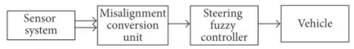
Sensor system Misalignment conversion unit Steering fuzzy controller Vehicle

Figure 5: Overall block diagram of the coil alignment system (ACAS).

transfer and efficiency and also increase the overall safety and comfort for the driver.

5. Concept of the ACAS

For the ACAS system, the hardware requirements are the electric power steering (EPS) system and sensors. The EPS is typically equipped in modern commercialized vehicles. The sensors are inexpensive and will detect the misalignment between the pick-up coil and power line. In general, the implementation of the ACAS system is inexpensive as it requires minimum hardware modifications, and it is mainly software implementation. The overall block diagram of the ACAS is shown in Figure 5.

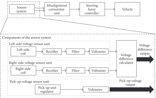
There are three subsystems in the ACAS, which consist of the sensor system, misalignment conversion unit, and the steering fuzzy controller. There are two outputs from the sensor system: the output value of the difference between two sensors that are installed on the left-side and right-side of the pick-up coil and the output value of the sensor installed at the pick-up coil regulator’s output. The two output values are received by the conversion unit, which will determine the lateral alignment value between the pick-up coil and power line. The alignment value is received by the steering fuzzy controller, where the necessary steering command will be sent to the EPS system of the vehicle.

5.1. Sensor System for the ACAS. The sensor system plays a crucial role in the ACAS system, and its block diagram is shown in Figure 6. There are three main sensor units: left-side voltage sensor unit, right-side voltage sensor unit, and the pick-up voltage sensor unit. The voltage difference between the left-side and right-side voltage sensor unit outputs is

(5)

Sensor system Misalignment conversion unit Steering fuzzy controller Vehicle Left-side coil Right-side coil Pick-up unit regulator Components of the sensor system

Rectifier Filter Voltmeter

Voltmeter Rectifier Filter Voltmeter Left-side voltage sensor unit

Right-side voltage sensor unit

Pick-up voltage sensor unit

Voltage difference calculator Pick-up voltage output Voltage difference output

Figure 6: Block diagram of the ACAS sensor system.

Pick-up coil

Front

Rear

Left-side coil Right-side coil x

y z

Figure 7: Diagram of left-side coil and right-side coil placement on pick-up coil shown in top view.

calculated by the voltage difference calculator. The calculated output and the output from the pick-up voltage sensor unit are sent to the misalignment conversion unit.

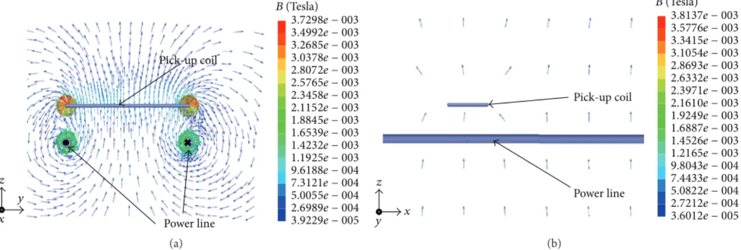
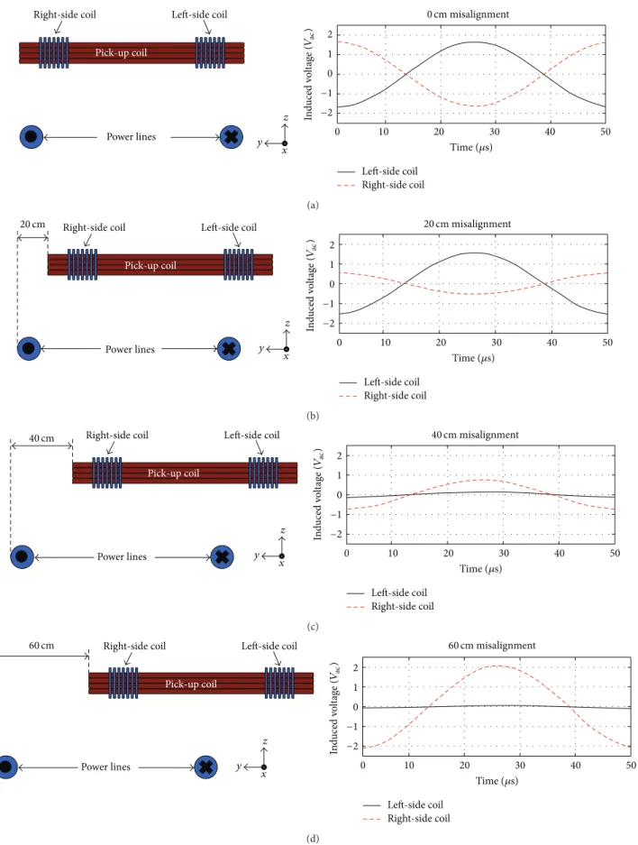
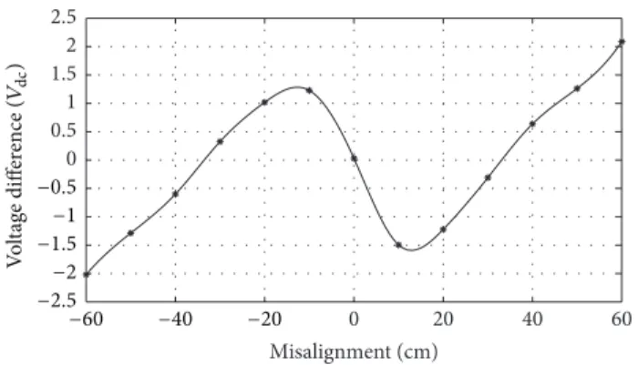
The main component of the pick-up voltage sensor unit is the DC voltmeter, which will measure the voltage output from the pick-up unit regulator. The components in the left-side voltage sensor unit and the right-left-side voltage sensor unit are the same; it consists of the coil, rectifier, regulator, and voltmeter. The coils described as left-side coil and right-side coil are smaller coils that are wrapped around the pick-up coil, as shown in Figure 7. The two coils are wrapped around the front side of the pick-up coil while keeping enough separation gap between them.

The two coils can also be installed at the rear side of the pick-up coil, but they must be installed along the front or the rear of the pick-up coil because of the magnetic flow direction between the power-line and pick-up coil apparent in the simulation results shown in Figure 8.

Figures 8(a) and 8(b) show the magnetic flow direction in front view and side view, respectively. While significant magnetic flow is visible from the front view, the magnetic flow from the side view is minimal. Even if the required voltage from the two coils is small, the induced voltage from the two coils if installed on the left/right side of the pick-up coil will be near zero volts, which is not desired.

The number of turns and the coil length of the left-side coil and the right-side coil should be kept at minimum, just enough to induce a voltage that can be read by the voltmeter. With bigger turns and bigger length of the two coils, it can disrupt the magnetic flow between the power line and pick-up coil, thus reducing the power transfer efficiency. In this paper, the two coils have been designed to have lengths of 7 cm with 25 turns, which were just enough to induce voltage within 2.5 V while not affecting the power transfer between the power line and pick-up coil. While using the model shown in Figure 3 as a basis, the two coils with the mentioned parameters were implemented and simulation was conducted. The simulation results are shown in Figure 9. Based on the results shown in Figure 9(a) through Figure 9(d), it shows how the voltage of the left-side coil and right-side coil varies as alignment is increased from 0 cm to 60 cm. However, the output voltage is in AC, where the difference between the two coils cannot be easily identified. Therefore, the two output waveforms are rectified and regu-lated into DC voltage, which can be read by the DC voltmeter. The resultant DC voltage output is then sent into the voltage difference calculator, where it is calculated as follows:

𝑉𝑑= 𝑉𝑙− 𝑉𝑟. (7)

𝑉_𝑙,𝑉_𝑟are the DC voltage readings from the left-side coil

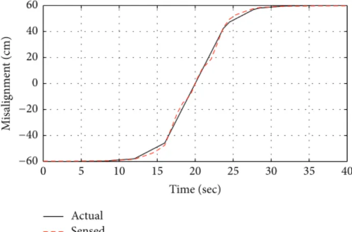
volt-age sensor unit and right-side coil sensor unit, respectively. The resultant voltage difference between the two coils relative to its alignment is shown in Figure 10.

(6)

Pick-up coil Power line x y z 3.9229e − 005 2.6989e − 004 5.0055e − 004 7.3121e − 004 9.6188e − 004 1.1925e − 003 1.4232e − 003 1.6539e − 003 1.8845e − 003 2.1152e − 003 2.3458e − 003 2.5765e − 003 2.8072e − 003 3.0378e − 003 3.2685e − 003 3.4992e − 003 3.7298e − 003 B (Tesla) (a) Pick-up coil Power line x y z 3.6012e − 005 2.7212e − 004 5.0822e − 004 7.4433e − 004 9.8043e − 004 1.2165e − 003 1.4526e − 003 1.6887e − 003 1.9249e − 003 2.1610e − 003 2.3971e − 003 2.6332e − 003 2.8693e − 003 3.1054e − 003 3.3415e − 003 3.5776e − 003 3.8137e − 003 B (Tesla) (b)

Figure 8: Maxwell simulation results showing the magnetic flow between the power line and pick-up coil from (a) front view and (b) side view.

However, based on the results shown in Figure 10, the nonlinear relationship between lateral misalignment and voltage difference can be observed, where the voltage differ-ence reading can imply left or right misalignment simulta-neously. This makes it difficult to determine the exact lateral misalignment location. Therefore, the voltage reading of the pick-up coil is needed in order to determine the exact lateral misalignment location, which is implemented as input for the misalignment conversion unit.

5.2. Misalignment Conversion Unit for the ACAS. The mis-alignment conversion unit shown in Figure 11 will change the nonlinear characteristic between the left-coil/right-coil voltage difference and the lateral misalignment into a more linear characteristic. It consists of the region selector unit, which divides the voltage difference readings into several regions. Each region consists of a model that has the linear

relationship between the voltage difference of the left-coil and right-coil voltage sensor unit, which can be mathematically expressed as follows:

𝑚_𝑛= 𝑦max(𝑛)− 𝑦min(𝑛)

𝑉𝑑 max(𝑛)− 𝑉𝑑 min(𝑛). (8)

𝑚_𝑛 refers to the slope of the specific linear region which

is identified as 𝐴, 𝐵, or 𝐵󸀠 and can go up to 𝑛 regions

depending on how many linear regions can be sectioned from the nonlinear voltage difference/lateral misalignment

relationship.𝑦_max(𝑛),𝑦_min(𝑛),𝑉_{𝑑 max(𝑛)}, and𝑉_{𝑑 min(𝑛)}refer to

the maximum and minimum lateral alignment distance and

voltage difference of a specific 𝑛 region, respectively. The

corresponding specific region model is selected by the region selector switch when it meets the specific criteria as follows:

𝑚_𝑛 = { { { { { { { { { { { { { { { { { { { { { { { { { { { { { { { { { { { { { { { { { { { { { { { { { { { { { { { { { { { { { { { { { { { { { 𝐴, if 𝑉_𝐿(𝑡) > 𝑉_𝑇1 𝐵, if (𝑉_𝐿(𝑡) < 𝑉_𝑇1) , (𝑉_𝑑(𝑡) > 𝑉_𝑑(𝑡 − 1)) , (𝑉_𝐿(𝑡) > 𝑉_𝐿(𝑡 − 1)) 𝐵, if (𝑉_𝐿(𝑡) < 𝑉_𝑇1) , (𝑉_𝑑(𝑡) < 𝑉_𝑑(𝑡 − 1)) , (𝑉_𝐿(𝑡) < 𝑉_𝐿(𝑡 − 1)) 𝐵󸀠_{, if (𝑉} 𝐿(𝑡) < 𝑉𝑇1) , (𝑉𝑑(𝑡) > 𝑉𝑑(𝑡 − 1)) , (𝑉𝐿(𝑡) > 𝑉𝐿(𝑡 − 1)) 𝐵󸀠, if (𝑉_𝐿(𝑡) < 𝑉_𝑇1) , (𝑉_𝑑(𝑡) < 𝑉_𝑑(𝑡 − 1)) , (𝑉_𝐿(𝑡) < 𝑉_𝐿(𝑡 − 1)) ... 𝑛, if (𝑉_𝑇1< 𝑉_𝐿(𝑡) < 𝑉_𝑇𝑛) , (𝑉_𝑑(𝑡) > 𝑉_𝑑(𝑡 − 1)) , (𝑉_𝐿(𝑡) > 𝑉_𝐿(𝑡 − 1)) 𝑛, if (𝑉_𝑇1< 𝑉_𝐿(𝑡) < 𝑉_𝑇𝑛) , (𝑉_𝑑(𝑡) < 𝑉_𝑑(𝑡 − 1)) , (𝑉_𝐿(𝑡) < 𝑉_𝐿(𝑡 − 1)) 𝑛󸀠_{, if (𝑉} 𝑇1< 𝑉𝐿(𝑡) < 𝑉𝑇𝑛) , (𝑉𝑑(𝑡) > 𝑉𝑑(𝑡 − 1)) , (𝑉𝐿(𝑡) > 𝑉𝐿(𝑡 − 1)) 𝑛󸀠_{, if (𝑉} 𝑇1< 𝑉𝐿(𝑡) < 𝑉𝑇𝑛) , (𝑉𝑑(𝑡) < 𝑉𝑑(𝑡 − 1)) , (𝑉𝐿(𝑡) < 𝑉𝐿(𝑡 − 1)) . (9)

(7)

Power lines

Right-side coil Left-side coil

Pick-up coil x y z 0 cm misalignment Left-side coil Right-side coil −2 −1 0 1 2 0 10 20 30 40 50 Time (𝜇s) In d uced v o lt ag e ( Vac ) (a) Right-side coil Left-side coil

Pick-up coil Power lines x y z 20 cm 20 cm misalignment Left-side coil Right-side coil −2 −1 0 1 2 0 10 20 30 40 50 Time (𝜇s) In d uced v o lt ag e ( Vac ) (b) Power lines

Pick-up coil x y z 40 cm 40 cm misalignment Left-side coil Right-side coil −2 −1 0 1 2 0 10 20 30 40 50 Time (𝜇s) In d uced v o lt ag e ( Vac ) (c) Power lines

Pick-up coil x y z 60 cm 60 cm misalignment Left-side coil Right-side coil −2 −1 0 1 2 0 10 20 30 40 50 Time (_𝜇s) In d uced v o lt ag e ( Vac ) (d)

Figure 9: Diagram with alignment parameters (drawing not in scale) between pick-up coil and power line and simulation results showing the induced voltage from the left-side coil and right-side coil at (a) 0 cm, (b) 20 cm, (c) 40 cm, and (d) 60 cm misalignment position.

(8)

−2.5−2 −1.5−1 −0.5 0 0.5 1 1.5 2 2.5 −40 −60 −20 0 20 40 60 Misalignment (cm) V o lt ag e diff er ence ( Vdc )

Figure 10: Simulation results showing the relationship between voltage difference of left-coil and right-coil and misalignment position.

Sensor system Misalignment conversion unit Steering fuzzy controller Vehicle

Components of the misalignment conversion unit

Pick-up voltage input

Voltage difference input

Region selector unit

Region selector switch Misalignment output converter Regionn Voltage→ misalignment Region_n󳰀 ... RegionB RegionB󳰀 RegionA

Figure 11: Block diagram of the ACAS misalignment conversion unit.

𝑚𝑛 of the corresponding region will be selected depending

on the voltage threshold𝑉_𝑇1, voltage difference𝑉_𝑑, and the

measured voltage from the pick-up voltage sensor unit𝑉_𝐿.

In this paper, the number of regions is limited to region𝐴,

region 𝐵, and region 𝐵󸀠 as shown in Figure 12. The upper

graph in the figure is the same graph shown in Figure 10, and it can be seen that each region consists of a linear relationship characteristic between the voltage difference and the lateral misalignment.

The misalignment range for region𝐴 is roughly between

±17 cm, while regions 𝐵 and 𝐵󸀠_{range between}_{−60 cm and}

−18 cm and between 60 cm to 18 cm, respectively. If assuming

that region𝐴 is selected by the region selector unit, it means

that𝑉_𝐿is greater than the voltage threshold𝑉_𝑇1. If𝑉_𝐿is lower

than𝑉_𝑇1, the region selector unit will either select region𝐵

or region𝐵󸀠. As shown in the lower graph of Figure 12,𝑉_𝑇1

is approximately 175 volts, which will toggle from region𝐴 to

region𝐵 or region 𝐵󸀠s at±17 cm.

The region selector will determine whether to select

region 𝐵 or region 𝐵󸀠 based on the previous and current

output values of𝑉_𝐿and𝑉_𝑑. As shown in (9), there are two

identical conditions that can meet the criteria for each region.

If assuming that region𝐵 is selected by the region selector

unit, it could either mean that the previous value of 𝑉_𝐿

and𝑉_𝑑is greater or less than its current𝑉_𝐿and 𝑉_𝑑 values.

This implies that the pick-up coil is moving either away or

towards the power line in region𝐵, and the condition that

is moving towards the power line is always selected. The

final selected 𝑚_𝑛 value from the region selector unit will

(9)

In d uced v o lt ag e a t p ic k -−2 −1 0 1 2 0 50 100 150 200 0 20 40 60 −20 −40 −60 Lateral alignment (cm) 0 20 40 60 −20 −40 −60 Lateral alignment (cm) V o lt ag e diff er ence ( Vdc ) RegionB RegionB RegionB󳰀 RegionB󳰀 Region_A u p co il r egula to r ( Vdc )

Figure 12: Correlation between voltage difference and pick-up coil voltage in order to determine the regions for the ACAS misalignment conversion unit.

Actual Sensed −60 −40 −20 0 20 40 60 M is alignmen t (cm) 5 10 15 20 25 30 35 40 0 Time (sec)

Figure 13: Simulation results comparing actual misalignment (desired) and the actual value that have been converted through the ACAS misalignment conversion unit.

with the given voltage difference input in the voltage →

misalignment converter as shown in

𝑦 = 𝑚_𝑛𝑉_𝑑. (10)

To validate the feasibility of the misalignment conversion unit, a simulation model was designed in SIMULINK that replicates the equations shown in (8) to (10). The simulation begins with misalignment between the power line and the

pick-up coil at −60 cm and progresses up until it reaches

misalignment of 60 cm. The simulation results are shown in Figure 13. The dashed line is the desired lateral alignment value versus time, and the bold line is the actual converted misalignment value by the misalignment conversion unit. Based on the results, it can be seen that at 0 to 17 sec and 22 to 40 sec range, the converted misalignment value has some

discrepancies with the desired misalignment value, where the maximum error recorded was around 5 cm. However, this is not of great significance as the fuzzy steering controller can compensate for the discrepancies and still achieve high performance to correct detected misalignment.

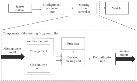
5.3. Steering Fuzzy Controller for the ACAS. The final sub-system of the ACAS sub-system is the steering fuzzy controller system as shown in Figure 14. Fuzzy control has been used to control the vehicle’s steering based on the misalignment reference given by the misalignment conversion unit. Fuzzy control has been used in various applications, such as energy management for hybrid vehicles, parking finding services, vehicle dynamics control, and many other applications [16– 19]. This control has also been applied to lane keeping assist systems (LKAS), which has similar resemblances to the fuzzy control specific for the ACAS [20, 21]. In addition, based on the reasons described in [18], fuzzy control method was specifically used for the ACAS application due to the nonlinear characteristics and the imprecise varying variables shown in Figures 12 and 13, respectively.

The received misalignment input is sent into the fuzzi-fication unit, where it is converted into two fuzzy inputs: misalignment and misalignment rate. Converting into a “fuzzy” value means that a “crisp” value, a value that is identified either as TRUE or FALSE, is converted into a value that can be both TRUE and FALSE. The values received as input are converted into a specific membership function (MF). Each MF is a set that contains a certain range of values. To convert into a “fuzzy” value, a triangular MF is used, and it is mathematically expressed as follows:

MF(triangle) = { { { { { { { { { { { { { { { { { { { 0 if 𝑥 ≤ 𝑎₁ 𝑥 − 𝑎₁ 𝑎₂− 𝑎₁ if 𝑎1< 𝑥 ≤ 𝑎2 𝑎₃− 𝑥 𝑎₃− 𝑎₂ if 𝑎2< 𝑥 ≤ 𝑎3 0 if 𝑎₃< 𝑥. (11)

𝑎₁ to𝑎₃ represent the𝑥 coordinates for the triangular MF,

where𝑎₁,𝑎₂, and𝑎₃ represent the left vertex, center vertex,

and right vertex of the triangle, respectively. 𝑥 is the value

received as an input from the fuzzy logic system before it goes through the “fuzzification” unit. However, there are certain situations where the input value is desired more as a “crisp” value than a “fuzzy” value. In this case, a trapezoidal MF is used, which is mathematically expressed as follows:

MF(trapezoid) = { { { { { { { { { { { { { { { { { { { { { { { { { 0 if 𝑥 ≤ 𝑏₁ 𝑥 − 𝑏₁ 𝑏₂− 𝑏₁ if 𝑏1< 𝑥 ≤ 𝑏2 1 if 𝑏₂< 𝑥 ≤ 𝑏₃ 𝑏4− 𝑥 𝑏₄− 𝑏₃ if 𝑏3< 𝑥 ≤ 𝑏4 0 if 𝑏₄< 𝑥. (12)

(10)

Misalignment Decision making unit Rule base Defuzzification unit Steering output Components of the steering fuzzy controller

Sensor system Misalignment conversion unit Steering fuzzy controller Vehicle Misalignment input Misalignment rate Fuzzification unit

Figure 14: Block diagram of the ACAS steering fuzzy controller.

SN OKAY SP POS NEG −0.5 0 0.5 1 1.5 −1 −1.5 1 0.5 0 (a) NONE POS NEG −0.2 −0.3 −0.1 0 0.1 0.2 0.3 1 0.5 0 (b)

Figure 15: Fuzzy input set for (a) lateral displacement and (b) lateral displacement rate.

𝑏₁to𝑏₄represent the𝑥 coordinates for the trapezoidal MF,

where𝑏₁,𝑏₂,𝑏₃, and𝑏₄represent the left vertex, left-center

vertex, right-center vertex, and right vertex of the trapezoid, respectively. Both the triangular and trapezoidal MFs have been used for the ACAS fuzzy logic controller, and the MF set for the lateral misalignment and its rate are shown in Figures 15(a) and 15(b), respectively.

In Figure 15(a), five MFs are defined: NEG (negative), SN (small negative), OKAY, SP (small positive), and POS (positive). Each MF has a specific misalignment range, while

the overall set ranges between −1.5 m and 1.5 m, which is

the maximum left or right position of one lane, respectively. The SN, OKAY, and SP MFs are put closer together with each other, while the NEG MF and the POS MF are put further away. This is to allow more sensitivity in control

within the −1.1 m to 1.1 m range. However, with increased

sensitivity, this may increase the oscillation of the system. To avoid this, another fuzzy input, which is the misalignment error rate, is implemented as shown in Figure 15(b). Three MFs are defined: NEG (negative), NONE, and POS (positive). The NEG and POS are trapezoidal MFs while the NONE is a triangular MF. This is to clearly define that the value is

negative or positive when the rate is below−0.2 m or above

0.2 m, respectively. NC R L SL SR 1 0.5 0 −0.6 −0.3 −0.9 0 0.3 0.6 0.9

Figure 16: Fuzzy output set for the ACAS fuzzy controller.

The fuzzy output block is shown in Figure 16, which will send the final “crisp” value command to the EPS unit of the vehicle. 5 MFs are defined: L (left), SL (small left), NC (no change), SR (small right), and R (right). The MFs range

from−0.9 to 0.9, which is the percentage of steering angle.

Although it is designed to have maximum steering command,

the steering output will not go more than±10 degrees due

to the given design constraints of the two fuzzy inputs and the rule base. This is an ideal case for the vehicle because it

(11)

Power line segment 1

Power line segment 2 Power line segment 3

0.1 m 0.3 m 1000 m 20 m 20 m 300 m 300 m 300 m

Figure 17: Diagram showing the placement of power lines on the road for SIMULINK and CarSim simulation.

will prevent any extreme steering situations, which is highly dangerous during high speed operations.

Rule Base for the Fuzzy Controller

(1) If “misalignment” is OKAY than “steering” is NC. (2) If “misalignment” is POS then “steering” is R. (3) If “misalignment” is SP then “steering” is SR. (4) If “misalignment” is SN then “steering” is SL. (5) If “misalignment” is NEG then “steering” is L. (6) If “misalignment” is OKAY and “rate” is POS then

“steering” is SL.

(7) If “misalignment” is OKAY and “rate” is NEG then “steering” is SR.

The rule base shown in the above list is what defines the boundaries of the fuzzy logic controller. It determines the degree of membership of each MF of its fuzzy input sets through the decision-making unit. The degree of

member-ship on both𝑦-axes of the two fuzzy inputs will define how

close the relationship is between each MF of its fuzzy set and the rule base. If degree of membership is closer to 1, it means that the relationship is strong, while 0 states the opposite. For example, if looking at the first rule set, it is defined that “misalignment” is OKAY. If the vehicle was positioned at the 0 cm mark, this would mean that the OKAY MF at the misalignment fuzzy input set will have a “1” degree of membership. This degree of membership ranging from 0 to 1 is used to determine the “cut-line” for the output fuzzy set. For example, if the degree of membership was at 0.7, this would mean that the corresponding fuzzy output set will have a “cut-line” at 0.7, where all area above the 0.7 threshold is ignored. From here, the final “crisp” steering output ratio, 𝛿, will be determined in the defuzzification unit using the Center of Gravity (COG) method as shown in (13). The COG

finds the center of area which is all output MFs𝑥 that are

located within the corresponding fuzzy output set with the

“cut-line,”𝑢_𝐴, within the intervals of𝑎 and 𝑏. 𝑎 and 𝑏 are the

corresponding𝑥-axis limits of the fuzzy output set:

𝛿 = ∫

𝑏

𝑎 𝑢𝐴(𝑥) 𝑥 𝑑𝑥

∫_𝑎𝑏𝑢_𝐴(𝑥) 𝑥 . (13)

Table 2: Parameters for vehicle model in CarSim.

Parameter Value

Model name C-Class, hatchback

Sprung mass 1274 kg Length 3.35 m Wheelbase 2.58 m Width 1.74 m Height 1.48 m Power 125 kW Tire 205/55 R16

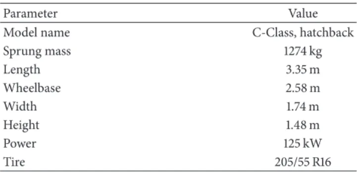
To evaluate the response of the steering fuzzy controller, as well as its ability to keep the vehicle within the power line, a simulation was conducted using SIMULINK and CarSim. To conduct the simulation, a road model similar to the diagram as shown in Figure 17 was designed, where the three power line segments of 300 m length were installed 20 m apart in a 1000 m road lane. The first power line segment was installed at the center of the road, and the second and third power line segments were deviated 0.3 m and 0.1 m from the center of lane, respectively. The vehicle model with the ACAS fuzzy steering controller was also designed as well. The vehicle model name and its parameters used in SIMULINK/CarSim simulation are shown in Table 2. The fuzzy steering con-troller was tested at four different speeds from 80 km/h up to 140 km/h in 20 km/h increments. This was to observe how well the ACAS fuzzy steering controller maintains its performance as the vehicle’s speed was increased.

Figure 18 shows the results of the simulation, where Figure 18(a) shows the lateral versus longitudinal displace-ment of the vehicle during the simulation. The thickest dash line is the desired position, which is the location of the three power lines. The other lines show the lateral versus longitudinal displacement of the vehicle at 80 km/h, 100 km/h, 120 km/h, and 140 km/h. Based on the result, the fuzzy steering controller was able to maintain its position near the desired lateral alignment position, even with increasing speeds.

Figure 18(b) shows the steering angle position of the fuzzy steering controller for the four different vehicle speeds. It can be seen that as vehicle speed increases, the oscillation

(12)

−0.05 0 0.05 0.1 0.15 0.2 0.25 0.3 0.35 L at eral disp lacemen t (m) 100 200 300 400 500 600 700 800 900 1000 0 Longitudinal displacement (m) 140 km/h 120 km/h 100 km/h Desired 80 km/h (a) 140 km/h 120 km/h 100 km/h80 km/h 5 10 15 20 25 30 35 40 45 0 Time (sec) −6 −4 −2 0 2 4 6 St eer a n gl e (deg) (b) −0.2 −0.15−0.1 −0.05 0 0.05 0.1 0.15 0.2 0.25 0.3 L at eral dist an ce er ro r (m) 140 km/h 120 km/h 100 km/h80 km/h 5 10 15 20 25 30 35 40 45 0 Time (sec) (c)

Figure 18: Simulation results showing the performance of steering fuzzy controller (a) lateral versus longitudinal displacement, (b) steering angle, and (c) lateral displacement error.

of the steering remained for a longer duration of the time. However, the remaining oscillation of the steering angle was very small, which was less than 1 degree. In addition, as illustrated in Figure 18(b), the maximum steering angle was at 6 degrees for all four vehicle speeds. This states that the vehicle’s dynamic was still stable enough or the vehicle would not have been able to maintain its desired path as shown in the results in Figure 18(a). Figure 18(c) shows the lateral displacement error between the desired and actual lateral position. Even with small steering angles, the vehicle was able to position its correct lateral position within 3 to 5 seconds once a significant lateral alignment error was detected, even at higher speeds. Overall, the results shown in Figure 18 validate the performance of the steering fuzzy controller.

6. Comparison Analysis

The operational validity of each subsystem in the ACAS, the sensor system, misalignment conversion unit, and the steer-ing fuzzy controller have been validated through simulation and show that each subsystem has performed as expected.

To view the feasibility of the overall ACAS system, the mitigation of power transfer loss due to misalignment was evaluated. To do so, another simulation was performed using SIMULINK and CarSim. Two vehicles, one vehicle with the ACAS controller and another vehicle without the ACAS controller, were operated on the same road shown in Figure 17. The first vehicle model is identical to the vehicle model used to test the steering fuzzy controller performance. The second vehicle is without the fuzzy controller model; it will only try to maintain the vehicle at the center of the road lane. This simulates a similar situation where the driver will operate the vehicle’s steering to maintain the vehicle at the center of the road lane as the driver assumes that the power line is at the center of the road.

Figure 19 shows the results of the simulation, where Figure 19(a) shows the amount of power being transferred to the pick-up coil in the vehicle. At 0 cm misalignment posi-tion, the two vehicles receive maximum power at 47.83 kW based on the analysis conducted in Figure 4. However, as the vehicles pass towards power lines 2 and 3, only the vehicle with the ACAS was able to retain most of the maximum power delivery, while the vehicle without ACAS could only

(13)

With ACAS Without ACAS 0 5 10 15 20 25 P o w er tra n sf er re d (kW) 5 10 15 20 25 30 35 40 45 0 Time (sec) (a) Max With ACAS Without ACAS 0 0.1 0.2 0.3 0.4 Ener g y acc u m u la te d (kW h ) 5 10 15 20 25 30 35 40 45 0 Time (sec) (b)

Figure 19: Simulated results showing amount of power transferred to vehicle with/without ACAS (a) and (b) accumulated energy to the vehicle due to power transfer.

receive roughly 4.90 kW and 26.35 kW of power at power lines 2 and 3, respectively.

Figure 19(b) shows the accumulated energy from the transferred power during the simulation time. As shown in the graph, the vehicle with the ACAS was able to accumulate about 578 Wh of energy at the end of the simulation, which is approximately 97% of the total maximum energy at 596 Wh. This maximum energy could have been accumulated only if the vehicle was at perfect alignment with the power line at all times. In case of the vehicle without the ACAS, the vehicle was only able to accumulate 311 Wh of energy at the end of the simulation, which is approximately 52% of the maximum energy that could be accumulated.

7. Conclusion

In this paper, an autonomous coil alignment system (ACAS) for vehicles with dynamic wireless charging is proposed. This system can detect lateral misalignment through three voltage sensors installed near the pick-up coil of the vehicle, and the nonlinear relationship between the voltage difference and misalignment position is converted into a more linear characteristic through the misalignment conversion unit. The lateral misalignment output from the misalignment conversion unit is received by the steering fuzzy controller, where the steering command is given to the electric power steering (EPS) system to control the vehicle’s lateral posi-tion. The performance and operational feasibility of each subsystem have been verified through various simulations. In

the comparison analysis, it shows that the vehicle equipped with ACAS improves the wireless power transfer efficiency, allowing the vehicle to receive maximum power 97% of the time. With improved pick-up coil designs in electric vehicles with dynamic wireless charging, combination of the ACAS system will certainly provide significant benefits as it will be able to retain near maximum power transfer capacity during operation, thus improving the overall power transfer efficiency for the vehicle.

Conflict of Interests

The authors declare that there is no conflict of interests regarding the publication of this paper.

Acknowledgment

This work was supported by the IT R&D program of MSIP/IITP (B0138-15-1002, study on the EMF exposure control in smart society).

References

[1] S. Nako, K. Okuda, K. Miyashiro, K. Komurasaki, and H. Koizumi, “Wireless power transfer to a microaerial vehicle with a microwave active phased array,” International Journal of

Antennas and Propagation, vol. 2014, Article ID 374543, 5 pages,

2014.

[2] H. Zhou, B. Zhu, W. Hu, Z. Liu, and X. Gao, “Modelling and practical implementation of 2-coil wireless power systems,”

Journal of Electrical and Computer Engineering, vol. 2014, Article

ID 906537, 8 pages, 2014.

[3] A. E. Rendon-Nava, J. A. D´ıaz-M´endez, L. Nino-de-Rivera, W. Calleja-Arriaga, F. Gil-Carrasco, and D. D´ıaz-Alonso, “Study of the effect of distance and misalignment between magnetically coupled coils for wireless power transfer in intraocular pressure measurement,” The Scientific World Journal, vol. 2014, Article ID 692434, 11 pages, 2014.

[4] M. A. Adeeb, A. B. Islam, M. R. Haider, F. S. Tulip, M. N. Ericson, and S. K. Islam, “An inductive link-based wireless power transfer system for biomedical applications,” Active and

Passive Electronic Components, vol. 2012, Article ID 879294, 11

pages, 2012.

[5] S. Kim, H.-H. Park, J. Kim, J. Kim, and S. Ahn, “Design and analysis of a resonant reactive shield for a wireless power electric vehicle,” IEEE Transactions on Microwave Theory and

Techniques, vol. 62, no. 4, pp. 1057–1066, 2014.

[6] A. Zaheer, H. Hao, G. A. Covic, and D. Kacprzak, “Investigation of multiple decoupled coil primary pad topologies in lumped IPT systems for interoperable electric vehicle charging,” IEEE

Transactions on Power Electronics, vol. 30, no. 4, pp. 1937–1955,

2015.

[7] T. Imura and Y. Hori, “Maximizing air gap and efficiency of magnetic resonant coupling for wireless power transfer using equivalent circuit and Neumann formula,” IEEE Transactions on

Industrial Electronics, vol. 58, no. 10, pp. 4746–4752, 2011.

[8] S. Raabe, G. A. J. Elliott, G. A. Covic, and J. T. Boys, “A quadrature pickup for inductive power transfer systems,” in

Proceedings of the 2nd IEEE Conference on Industrial Electronics and Applications (ICIEA ’07), pp. 68–73, IEEE, May 2007.

(14)

[9] M. L. G. Kissin, G. A. Covic, and J. T. Boys, “Steady-state flat-pickup loading effects in polyphase inductive power transfer systems,” IEEE Transactions on Industrial Electronics, vol. 58, no. 6, pp. 2274–2282, 2011.

[10] G. A. J. Elliott, S. Raabe, G. A. Covic, and J. T. Boys, “Multiphase pickups for large lateral tolerance contactless power-transfer systems,” IEEE Transactions on Industrial Electronics, vol. 57, no. 5, pp. 1590–1598, 2010.

[11] J. Shin, S. Shin, Y. Kim et al., “Design and implementation of shaped magnetic-resonance-based wireless power transfer system for roadway-powered moving electric vehicles,” IEEE

Transactions on Industrial Electronics, vol. 61, no. 3, pp. 1179–

1192, 2014.

[12] S. Ahn, N. Suh, and D.-H. Cho, “Charging up the road,” IEEE

Spectrum, vol. 50, no. 4, pp. 48–54, 2013.

[13] Y. D. Ko and Y. J. Jang, “The optimal system design of the online electric vehicle utilizing wireless power transmission technology,” IEEE Transactions on Intelligent Transportation

Systems, vol. 14, no. 3, pp. 1255–1265, 2013.

[14] S. Shin, J. Shin, Y. Kim et al., “Hybrid inverter segmentation control for online electric vehicle,” in Proceedings of the IEEE

International Electric Vehicle Conference (IEVC ’12), Greenville,

SC, USA, March 2012.

[15] S. Lukic and Z. Pantic, “Cutting the cord: static and dynamic inductive wireless charging of electric vehicles,” IEEE

Electrifi-cation Magazine, vol. 1, no. 1, pp. 57–64, 2013.

[16] Z. Chen, J. C. Xia, and B. Irawan, “Development of fuzzy logic forecast models for location-based parking finding services,”

Mathematical Problems in Engineering, vol. 2013, Article ID

473471, 6 pages, 2013.

[17] G. Yin, S. Wang, and X. Jin, “Optimal slip ratio based fuzzy control of acceleration slip regulation for four-wheel inde-pendent driving electric vehicles,” Mathematical Problems in

Engineering, vol. 2013, Article ID 410864, 7 pages, 2013.

[18] N. J. Schouten, M. A. Salman, and N. A. Kheir, “Fuzzy logic control for parallel hybrid vehicles,” IEEE Transactions on

Control Systems Technology, vol. 10, no. 3, pp. 460–468, 2002.

[19] J. Chien, J. Lee, and L. Liu, “A fuzzy rules-based driver assistance system,” Mathematical Problems in Engineering, vol. 2015, Article ID 207675, 14 pages, 2015.

[20] J. E. Naranjo, C. Gonz´alez, R. Garc´ıa, and T. De Pedro, “Lane-change fuzzy control in autonomous vehicles for the overtaking maneuver,” IEEE Transactions on Intelligent Transportation

Systems, vol. 9, no. 3, pp. 438–450, 2008.

[21] G. Wang, J. Zhao, X. Zhang, and R. Zhao, “Multi-model fuzzy controller for vehicle lane tracking,” in Proceedings of the IEEE

17th International Conference on Intelligent Transportation Sys-tems (ITSC ’14), pp. 1341–1346, IEEE, Qingdao, China, October

(15)