경북대학교 에너지화공전공

1

Chapter 13.

Chemical-Reaction Equilibria

• The transformation of raw materials into products of greater value by means of chemical reaction is a major industry, and a vast array of commercial products is obtained by chemical synthesis.

• Sulfuric acid, ammonia, ethylene, propylene, phosphoric acid, chlorine, nitric acid, urea, benzene, methanol, ethanol, and ethylene glycol are examples of chemicals produced in the United States in billions of kilograms each year.

 These in turn are used in the large-scale manufacture of fibers, paints, detergents, plastics, rubber, paper, fertilizers, insecticides, etc.

• Clearly, the chemical engineer must be familiar with chemical-reactor design and operation.

• Both the rate and the equilibrium conversion of a chemical reaction depend on the temperature, pressure, and composition of reactants.

Lecture 1 2

• Consider, for example, the oxidation of sulfur dioxide to sulfur trioxide.  A catalyst is required if a reasonable reaction rate is to be attained.

 With a vanadium pentoxide catalyst the rate becomes appreciable at about 573.15 K (300°C) and continues to increase at higher temperatures.

 On the basis of rate alone, one would operate the reactor at the highest practical temperature.

 However, the equilibrium conversion to sulfur trioxide falls as temperature rises, decreasing from about 90% at 793.15 K (520°C) to 50% at about 953.15 K (680°C).

 These values represent maximum possible conversions regardless of catalyst or reaction rate.

• The evident conclusion is that both equilibrium and rate must be considered in the exploitation of chemical reactions for commercial purposes.

 Although reaction rates are not susceptible to thermodynamic

treatment, equilibrium conversions are.

• Therefore, the purpose of this chapter is to determine the effect of

temperature, pressure, and initial composition on the equilibrium conversions of chemical reactions.

Lecture 1 3

Lecture 1 4

Chemical-Reaction Equilibria

Both the rate and equilibrium conversion of a chemical

reaction depend on the temperature, pressure, and

composition of reactants.



Although reaction rates are not susceptible to

thermodynamic

treatment,

equilibrium

conversions are.



The purpose of this lecture is to determine the effect

of temperature, pressure, and initial composition

on the equilibrium conversions of chemical

• Reaction stoichiometry is treated in Sec. 13.1 • reaction equilibrium, in Sec. 13.2.

• The equilibrium constant is introduced in Sec. 13.3,

• its temperature dependence and evaluation are considered in Secs. 13.4 and 13.5.

• The connection between the equilibrium constant and composition is developed in Sec. 13.6.

• The calculation of equilibrium conversions for single reactions is taken up in Sec. 13.7.

• In Sec. 13.8, the phase rule is reconsidered; • Multireaction equilibrium is treated in Sec. 13.9.

• finally, in Sec. 13.10 the fuel cell is given an introductory treatment.

A general chemical reaction:

 positive (+)for products and negative (-)for reactants

 the stoichiometric numbers are:

...

...

_{3 3 4 4} 2 2 1 1

A



v

A





v

A



v

A



v

13.1 Reaction coordinate

; stoichiometric coefficient A_i ; chemical formula. ν_i ; stoichiometric numbers 1 v (13.1)

• The stoichiometric number for an inert species is zero.

• For the reaction represented by Eq. (13.1), the changes in the numbers of moles of the species present are in direct proportion to the stoichiometric numbers.

 Thus for the preceding reaction, if 0.5 mol of CH₄ disappears by reaction, 0.5 mol of H₂O must also disappear; simultaneously 0.5 mol of CO and 1.5 mol of

H₂ are formed. 4 2 1( 0.5 ) 2( 1.5 ) _{( 0.5)} ( 1) ( 3) CH H dn dn d v v    _   _{ }   

• Applied to a differential amount of reaction, this principle provides the equations:

• It has the advantage that the change in the extent of reaction dε is the same for each component,

 whereas the changes in the number of moles are different for different species taking part in the reaction.

• The general relation between a differential change dn_i in the number of moles of a reacting species and dε is therefore

• Equations (13.2) and (13.3) define changes in ε with respect to changes in the numbers of moles of the reacting species.



d

v

dn

v

dn

v

dn

v

dn

_

_

_

_

_

...

4 4 3 3 2 2 1 1

)

...,

,

2

,

1

(

i

N

d

v

dn

_i



_i





Reaction coordinate

(13.2) (13.3) 4 2 1( 0.5 ) 2( 1.5 ) _{( 0.5)} ( 1) ( 3) CH H dn dn d v v    _   _{ }   

• Reaction coordinate ε ; characterizes the extent or degree to which a reaction has taken place.

• The definition of ε itself is completed for each application by setting it equal to zero for the initial state of the system prior to reaction.

)

...,

,

2

,

1

(

i

N

d

v

dn

_i



_i





Reaction coordinate

 The ν_i are pure numbers without units; Eq. (13.3) therefore requires ε to be expressed in moles.

 This leads to the concept of a mole of reaction, meaning a change in ε of one mole.

 When △ε = 1 mol, the reaction proceeds to such an extent that the change in

mole number of each reactant and product is equal to its stoichiometric number.

i i i i

n

v

n

v



  

 

(13.3) i i dn d v  

 Thus, integration of Eq. (13.3) from an initial unreacted state where ε = 0 and n_i = n_i0, to a state reached after an arbitrary amount of reaction gives:

Reaction coordinate

0 0 0 0 ( 1, 2, ..., ) ( 1, 2, ..., ) i i n i i n i i i i i i dn v d i N n n v n n v i N 







      





0 0 i i i i i i n n n v n v       







0 0 i i i i i _total n n v n y n n v n       

)

...,

,

2

,

1

(

i

N

d

v

dn

_i



_i





(13.3)

Summation over all species yields:

Thus the mole fractions y_i of the species present are related to ε by:

(13.5) (13.4)

Example 13. 1 For a system in which the following reaction occurs,

assume there are present initially 2 mol CH₄, 1 mol H₂O, 1 mol CO and 4 mol H₂. Determine expressions for the mole fractions y_i as functions of ε.

2

3

1

1

1

















i i





4 2 2 CH + H O  CO + 3H





v

n

v

n

n

n

y

i i i i









0 0

2

1

1

4

8

0 0















i i

n

n





2

8

2

4







CH

y





2

8

1







CO

y





2

8

1

2







O H

y





2

8

3

4

2







H

y

 The mole fractions of the species in the reacting mixture are seen to be functions of the single variable ε.

initially

4 2 2

CH + H O



CO + 3H

0

8 2

Example 13. 1 For a system in which the following reaction occurs,

assume there are present initially 3 mol CH₄, 2 mol H₂O. Determine expressions for the mole fractions y_i as functions of ε.

2

3

1

1

1

















i i





4 2 2 CH + H O  CO + 3H





v

n

v

n

n

n

y

i i i i









0 0 0 i0

3 2 0 0 5

i

n





n

    

4

3

5 2

CH

y











0

5 2

CO

y











2

2

5 2

H O

y











2

0 3

5 2

H

y











 The mole fractions of the species in the reacting mixture are seen to be functions of the single variable ε.

initially

4 2 2

CH + H O



CO + 3H

0

5 2

Example 13. 2 Consider a vessel which initially contains only n₀ mol of water vapor. If decomposition occurs according to the reaction,

find expressions which relate the number of moles and the mole fraction of each chemical species to the reaction coordinate ε.

2 1 2 1 1 1     



i i   2 2 2 2 1 O H O H  





v

n

v

n

n

n

y

i i i i

_







0 0 0 0 0 n n n i i  



  2 1 0 0 2    n n y_{H O} 2 0 0 1 2 H y n      2 0 1 0 2 1 2 O y n      2 0 ( 1) H O n  n    2 1 0 ( ) 2 O n     2 0 ( 1) H n     0 0 1 2 n n v n       Fractional decomposition of water vapor is:

2 0 _{0 0} 0 0 0 ( ) H O n n _{n n} n n n    _{ }  

when n₀=1, ε is identified with the fractional decomposition of water vapor

0( 0)

i i i

Multi-reaction Stoichiometry

• Two or more independent reactions proceed simultaneously  A separate reaction coordinate ε_j applies to each reaction.

 The stoichiometric numbers are doubly subscripted to identify their association with both a species and a reaction.

 ν_i,j : the stoichiometric number of species i in reaction j. • The change of the moles of a species n_i:

j j j i i

v

d

dn





_,







i j i j



,



total stoichiometric number:

j j j i i i

n

v

n



₀





_,



integration summation

 

0 , 0 , i i j j i j i i j j j i

n

n

v

n

v









 





 

j j j

v

n

n



₀







j j j j j j i i i

v

n

v

n

y















0 , 0 i i

dn



v d



0 0 , i j i n i i j j n j

dn







v d







) ..., , 2 , 1 ( 0 0 N i d v dn _i n n i i i  





  cf; ) ..., , 2 , 1 ( 0 v i N n n_i  _i  _i  ( i = 1, 2, ... , N ) reaction index 0 , i i i j _j n  n  v 







(13.6) (13.7)

Example 13.3 Consider a system in which the following reactions occur,

if there are present initially 2 mol CH₄ and 3 mol H₂O, determine expressions for the y_i as functions of ε₁ and ε₂ .

2 2 4 H O CO 3H CH    2 2 2 4 2H O CO 4H CH    j j j j j j i i i

v

n

v

n

y















0 , 0 2 1 2 1

2

2

5

2

4



















CH

y

4 4 4 4 2 0 , ,1 1 ,2 2 1 2 0 1 1 2 2 1

( 2 )

(

)

( 2 3)

(

)

i CH i j j CH CH j CH j j j

n

v

v

v

y

n

v

v

v













 











  









(1) (2)



 i j i j  ,  1 2 1 1 1 3 2 1 2 1 4 2 j i i j i i                      





0 i0 2 3 5 i n 



n    i CH₄ H₂O CO CO₂ H₂ j ν_j 1 -1 -1 1 0 3 2 2 -1 -2 0 1 4 2

2 1 2 1

2

2

5

2

3

2



















O H

y

2 1 1

2

2

5













CO

y

2 1 2

2

2

5

2













CO

y

2 1 2 1

2

2

5

4

3

2

















H

y

The composition of the system is a function of _{independent variables ε} 1 and ε2. 2 2 2 2 2 0 , ,1 1 ,2 2 1 2 0 1 1 2 2 1

( 3 )

(

)

( 2 3)

(

)

i H O i j j H O H O j H O j j j

n

v

v

v

y

n

v

v

v













 











  









2 2 4 H O CO 3H CH    2 2 2 4 2H O CO 4H CH   

Initially 2 mol CH₄,3 mol H₂O

2 1 2 1

2

2

5

2

4



















CH

y

i_j CH4 H2O CO CO2 H2 _νj 1 -1 -1 1 0 3 2 2 -1 -2 0 1 4 2

13.2 Application of Equilibrium criteria to chemical reactions

• The total Gibbs energy of a closed system at constant T and P must decrease

during an irreversible process and that the condition for equilibrium is reached when Gt _{attains its minimum value.}

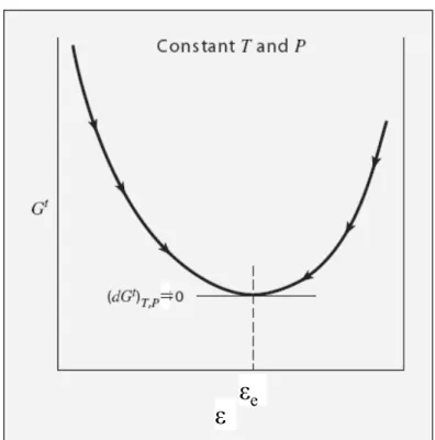
Figure 13.1 The total Gibbs energy in relation to the reaction coordinate

=

ε εe

• Thus if a mixture of chemical species is not in chemical equilibrium,

 any reaction that occurs at constant T and P must lead to a decrease in the total Gibbs energy of the system.

At this equilibrium state, _(dGt₎

13.2 Application of Equilibrium criteria to chemical reactions

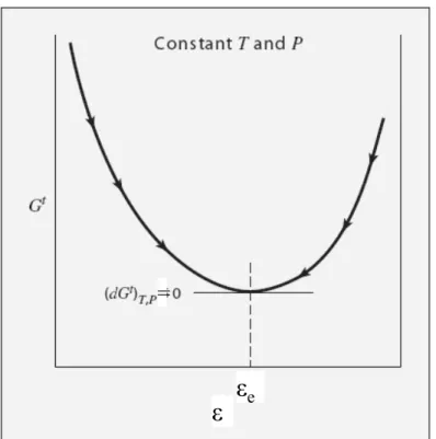
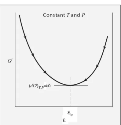
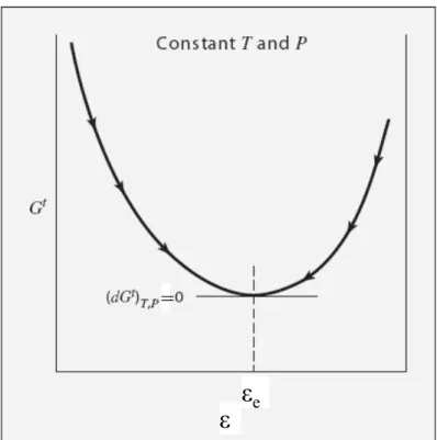
 The significance of this for a single chemical reaction is seen in Fig. 13.1, which shows a schematic diagram of Gt _{vs. ε, the reaction}

coordinate.

 Since ε is the single variable that characterizes the progress of the reaction, and therefore the composition of the system, the total Gibbs energy at constant T and P is determined by ε.

 The arrows along the curve in Fig. 13.1 indicate the directions of changes in (Gt₎

T,P

are possible on account of reaction.

(dGt₎

T,P=0

Figure 13.1 The total Gibbs energy in relation to the reaction coordinate

(14-64)

=

• The reaction coordinate has its equilibrium value ε_e, at the minimum of the curve.  The meaning of Eq. (14.64) is that differential displacements of the chemical

reaction can occur at the equilibrium state without causing changes in the total Gibbs energy of the system.

• Figure 13.1 indicates the two distinctive features of the equilibrium state for given temperature and pressure:

▪ The total Gibbs energy Gt _{is a minimum. ▪ Its differential is zero.}

 

_dGt _T,P  0

(14.64)

=

Figure 13.1 The total Gibbs energy in relation to the reaction coordinate

ε_e ε

• Each of these may serve as a criterion of equilibrium.

 Thus, we may write an expression for Gt _as

a function of ε and seek the value of ε which minimizes Gt_,

 or we may differentiate the expression, equate it to zero, and solve for ε .

 The latter procedure is almost always used for single reactions (Fig. 13.1), and leads to the method of equilibrium constants, as described in the following sections.

 It may also be extended to multiple reactions, but in this case the direct minimization of Gt _{is often more convenient,} and is considered in Sec. 13.9.

=

Figure 13.1 The total Gibbs energy in relation to the reaction coordinate

ε εe

• Although the equilibrium expressions are developed for closed systems at constant T and P, they are not restricted in application to systems that are actually closed and reach equilibrium states along paths of constant T and P.

 Once an equilibrium state is reached, no further changes occur, and the system continues to exist in this state at fixed T and P.

 How this state was actually attained does not matter. Once it is known that an equilibrium state exists at given T and P, the criteria apply.

13.3 Standard Gibbs energy change and the equilibrium constant









i i i

dn

dT

nS

dP

nV

nG

d

(

)

(

)

(

)



 d v dn_i  _i









i i i

d

dT

nS

dP

nV

nG

d

(

)

(

)

(

)







0

)

(

)

(

, ,

















































atequilibrium P T t P T i i i

G

nG









Equation (11.2), the fundamental property relation for single-phase systems, provides an expression for the total differential of the Gibbs energy:

(11.2)

Since nG is a state function, the right side of this equation is an exact differential expression

• Thus the quantity ∑ν_iμ_i represents, in general, the rate of change of the total Gibbs energy of the system with the reaction coordinate at constant T and P.

• Figure 13.1 shows that this quantity is zero at the equilibrium state. • A criterion of chemical-reaction equilibrium is therefore:

0

i i i

 







                       i i n T P i n P n T dn n nG dT T nG dP P nG nG d j , , , , ) ( ) ( ) ( ) ( (13.8)

The fugacity of a species in solution:

i i

i





(

T

)



RT

ln

f

ˆ



For pure species i in its standard state: _o

i i o i

T

RT

f

G





(

)



ln

o i i o i i

f

f

RT

G



ln

ˆ





0 



i i i 

0

ˆ

ln

_





















i _io i o i i

f

f

RT

G



ˆ

ln

0

i v o _i i i _o i i _i

f

G

RT

f







_



_











RT G f f _i i io i v o i i i





_         ˆ



ln

K

f

f

i v o i i i





















ˆ

( −

ˆ ln( ) 0 o o i i i i G RT f f  _{ } _{ }



3 1 2 3 1 2 1 2 3 ˆ ln 0 ˆ ln ˆ ˆ ˆ ln ln ln i i v o i i i o i i i o v i i i i o i i v v v o o o f G RT f G f f RT f f f f f f      _{ }                      _{ }                 









ˆ ln( ) o o i Gi RT f fi



  ˆ ln i v i o i i f f   _ _   ˆ exp exp i o v i i o i i o i i G f G K f RT RT       _{    } _{ }  _{ }  _{ }        _{ }



(13.9) (11.42) (13.10) 0 0 0 i i i G  G G  







 (13.12) (13.11a) ln o G K RT   (13.11b)

• Since G_io _{is a property of pure species i in its standard state at fixed pressure, it depends}

only on temperature.

 By Eq. (13.12) it follows that ∆Go _{and hence K, are also functions of temperature only.}

• In spite of its dependence on temperature, K is called the equilibrium constant for the reaction; ∑ν_i G_io_{, represented by ∆G}o _{, is called the standard Gibbs-energy change of}

reaction.

• The fugacity ratios in Eq. (13.10) provide the connection between the equilibrium state of interest and the standard states of the individual species, for which data are presumed available, as discussed in Sec. 13.5.

• The standard states are arbitrary, but must always be at the equilibrium temperature T.  The standard states selected need not be the same for all species taking part in a

reaction.

 However, for a particular species the standard state represented by G_io _{must be the} same state as for the fugacity f_io_.

o o o i i i i i G  G G  







 (13.10) (13.12) K f f i v o i i i         



ˆ ˆ exp exp i o v i i o i i o i i G f G K f RT RT      _{   } _{ }  _{ } _{ }       _{ }



• The function ∆Go _=∑ν

i Gioin Eq. (13.12) is the difference between the Gibbs energies

of the products and reactants (weighted by their stoichiometric coefficients) when each is in its standard state as a pure substance at the standard-state pressure, but at the system temperature.

 Thus the value of ∆Go _{is fixed for a given reaction once the temperature is}

established, and is independent of the equilibrium pressure and composition.  Other standard property changes of reaction are similarly defined. Thus, for the

general property M: o o o i i i i i G  G G  







 _(13.12) o o i i i

M



M







• In accord with this, △Ho_{is defined by Eq. (4.14) and △Cp}o_{; by Eq. (4.16).}

• These quantities are functions of temperature only for a given reaction, and are related to one another by equations analogous to property relations for pure species.

• For example, the relation between the standard heat of reaction and the standard Gibbs energy change of reaction may be developed from Eq. (6.39) written for species i in its standard state: dT RT G d RT H o i o i         2 dT RT G d RT H i o i i i o i i            









2 o o i i i H  H  



_Po _{i P}o_i i

C



C







Multiplication of both sides by v_i and summation over all species

        RT G K o exp

dT

RT

G

d

RT

H

i o i i i o i i

































2





dT

RT

G

d

RT

H

o o

_

_





2

dT

K

d

RT

H

o

ln

2





0 lnK G RT    _{  }   (13.13) o o i i i

M



M







o o i i i H  H  



o o i i i G  G  



,

13.4 Effect of Temperature on the Equilibrium Constant





dT RT G d RT H o o _{ }   2

dT

K

d

RT

H

o

ln

2





• Equation (13.14) gives the effect of temperature on the equilibrium constant, and hence on the equilibrium conversion.

• If ∆Ho _{is negative, i.e., if the reaction is exothermic, the equilibrium constant}

decreases as the temperature increases.

• Conversely, K increases with T for an endothermic reaction.

• If ∆Ho_{, the standard enthalpy change (heat) of reaction, is assumed}

independent of T,

 integration of Eq. (13.14) from a particular temperature T' to an arbitrary temperature T leads to the simple result:

(13.15)

(13.14)

• Since the standard-state temperature is that of the equilibrium mixture, the standard property changes of reaction, such as △G˚ and △H˚, vary with the equilibrium temperature. The dependence of △G˚ on T is given by Eq. (13.13)

(13.13)





2 o o G d _{RT H} dT RT    0 lnK G RT    _{  }   2 ' '

1

1

ln

,

ln

'

'

o o K T K T

H

dT

K

H

d

K

R

T

K

R

T

T





_

_



 

_



_









13.4 Effect of Temperature on the Equilibrium Constant ' ' 1 1 ln o K H K R T T      _  _  

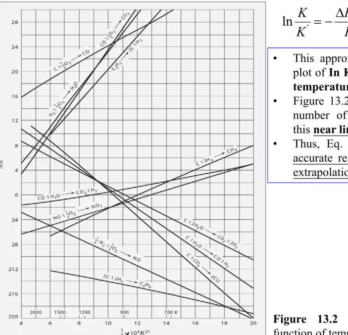
• This approximate equation implies that a plot of In K vs. the reciprocal of absolute

temperature is astraight line.

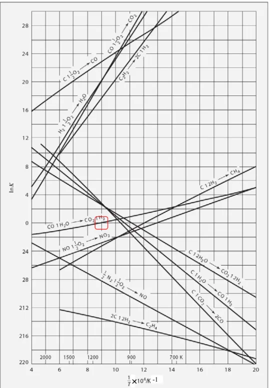
• Figure 13.2, a plot of In K vs. 1/T for a number of common reactions, illustrates this near linearity.

• Thus, Eq. (13.15) provides a reasonably accurate relation for the interpolation and extrapolation of equilibrium-constant data.

(13.15)

×

Figure 13.2 Equilibrium constants as a function of temperature

o i o i o i

H

TS

G











_i





_i i io o i i i o i i

G



H

T



S



o o o

_H

_T

_S

G











and summation













T T o P o o

_dT

R

C

R

H

H

0 0













T T o P o o

T

dT

R

C

R

S

S

0 0 0 0 0 0

T

G

H

S

o o o

_













0 0 0 0 0 0 0 0 0 0 0 0 0 0 ( ) o o o o o T T o P o P T T o o T T o o P P T T o o T T o o o P P T T G H T S C C dT H R dT T S R R R T C C dT H T S R dT RT R R T C C T dT H H G R dT RT T R R T                               













• The rigorous development of the effect of temperature on the equilibrium constant is based on the definition of the Gibbs energy, written for a chemical species in its standard state: Multiplication by ν_i (4.18) P P dT V dS C dP T T     _{  }   

At const. std. state pressure Po

o o o _{H T S} G      (13.18) (6-21) (13.17)





0 0 0 0 0 0 o o T T o o o o P P T T

T

C

C dT

G

H

H

G

R

dT RT

T

R

R

T







 





 









0 0 0 0 0 0

1

o o o o _T o _T o P P T T

G

G

H

H

C

C dT

dT

RT

RT

RT

T

R

R

T



_



 

_



_



_







1 ; RT       0 IDCPH(T0,T;DA,DB,DC,DD) o T P T C dT R  _



0 2 0 0 2 2 0

1

ln

(

1)

2

T P T

C dT

D

A

BT

CT

R T

T











_

_





_{ }

_{ }

_{ }

_



_



_

_







_



_













0 IDCPS(T0,T;DA,DB,DC,DD) o T P T C dT R T  



(13-18) 0 2 2 3 3 0 0 0 0

1

(

) (

1)

(

1)

(

1)

2

3

T P T

C

B

C

D

dT

A T

T

T

R

T













_{ }

_{ }



_{ }



_{ }



_



_











0 , , , i i i T T A A B C and D        



Thus

△

GO_{/RT(=-InK) as given by Eq. (13.18) is readily calculated at any}

temperature from the standard heat of reaction and the standard Gibbs-energy change of reaction at a reference temperature [usually 298.15 K (25˚C)], and from two functions which can be evaluated by standard computational procedures.





0 0 0 0 0 0 o o T T o o o o P P T T

T

C

C dT

G

H

H

G

R

dT RT

T

R

R

T







 





 









RT G K o   

ln Readily calculated at any temperature from the standard heat of reaction and the standard Gibbs energy change of reaction at a reference temperature.

2 1 0

K

K

K

K



        0 0 0 exp RT G K o                T T RT H K o 0 0 0 1 exp 1      _  _  





T T o P T T o P T dT R C dT R C T K 0 0 1 exp 2 0 0 0 0 0 0 0 0 0 0 0 0 0 0 0 0 0 0 0 0 0 1 0 0 0 ln ln 1 ln 1 o o o o _T o _T o P P T T o o o o o o o o o o T T T P P P T T T G H T H T G R C RT C dT K dT RT RT RTT RTT RT R RT R T T G G K RTT RT H T H H H H T K RT RTT RT RT RT T R C RT C dT C dT dT RT R RT R T T R                          _{ }       _  _            











0 2 ln o T P T C dT K R T 



• The first factor K₀ represents the equilibrium constant at reference temperature T₀

• The second factor K₁ is a multiplier that supplies the major effect of temperature, such that the product K₀K_l is the equilibrium constant at temperature T when the heat of reaction is assumed independent of temperature

• The third factor K₂ accounts for the much smaller temperature influence resulting from the change of ∆Ho _{with temperature:}

0 1 2

ln

ln

ln

ln

K

K

K

K









1 ; RT    _{ }  

Figure 13.2 Equilibrium constants as a function of temperature

• Values of ∆Go _{for many formation reactions are tabulated in standard reference.} • The reported values of ∆Go

f not measured experimentally, but are calculated by Eq. (13.16).

• The determination of ∆So

f ; may be based on the third law of thermodynamics, discussed in Sec. 5.10.

 Combination of values from Eq. (5.40) for the absolute entropies of the species taking part in the reaction gives the value of ∆So

f.

 Entropies (and heat capacities) are also commonly determined from statistical calculations based on spectroscopic data.

13.5 Evaluation of Equilibrium Constant

o o

o

_H

_T

_S

G









• Values of ∆Go

f298 or a limited number of chemical compounds are listed in Table C.4 of App. C.

 These are for a temperature of 298.15 K (25℃), as are the values of ∆Ho

f298 listed in the same table.

• Values of ∆Go _{for other reactions are calculated from formation-reaction} values in exactly the same way that ∆Ho _{values for other reactions are} determined from formation-reaction values (Sec. 4.4).

• In more extensive compilations of data, values of ∆Go

f and ∆Hof are given for a wide range of temperatures, rather than just at 298.15 K (25°C).

 Where data are lacking, methods of estimation are available; these are reviewed by Reid, Prausnitz, and Poling.

13.5 Evaluation of Equilibrium Constant

o o

o

_H

_T

_S

G









Example 13.4 Calculation the equilibrium constant for the vapor-phase hydration of ethylene at 145 and at 320 °C from data given in App.C.

2 4 2 2 5

C H +H O



C H OH

The heat capacity data:

2 1 0

K

K

K

K





C

₂

H

₅

OH

 



C

₂

H

₄

 



H

₂

O







        0 0 0 exp RT G K o                T T RT H K o 0 0 0 1 exp 1      _  _  





T T o P T T o P T dT R C dT R C T K 0 0 1 exp 2 From Table C.4

mol

J

H

H

₀o





₂₉₈o





45792



mol

J

G

G

₀o





₂₉₈o





8378



T K₀ K₁ K₂ K 298.15 29.366 1 1 29.366 418.15 29.366 4.985x10-3 _{0.986 1.443x10}-1 593.15 29.366 1.023x10-4 _{0.9794 2.942x10}-3 RT G K o    ln

        0 0 0 exp RT G K o                T T RT H K o 0 0 0 1 exp 1           





T T o P T T o P T dT R C dT R C T K 0 0 1 exp 2 RT G K o    ln 2 1 0

K

K

K

K



△H = △H -(△H + △H )

O R O f, C₂H₅OH O f, C₂H₄ Of, H₂O

C

₂

H

₄

(g) + H

₂

O(g) =>C

₂

H

₅

OH(g)

0 0 0 0 0 0

1

o o o o _T o _T o P P T T

G

G

H

H

C

C dT

dT

RT

RT

RT

T

R

R

T



_



 

_



_



_







Lecture 1 35 0 0 0 0 0 0

1

o o o o _T o _T o P P T T

G

G

H

H

C

C dT

dT

RT

RT

RT

T

R

R

T



_



 

_



_



_







K _RTG o    ln

For T=418.15 K 0 0 0 0 0 0 1 o o o o _T o _T o P P T T G G H H C C dT dT RT RT RT T R R T  _    _  _  _ 





0 2 0 0 2 2 0 1 ln ( 1) 2 T P T C dT D A BT CT R T T          _{      }  _  _{ }   _ _    



0 2 2 3 3 0 0 0 0 1 ( ) ( 1) ( 1) ( 1) 2 3 T P T C B C D dT A T T T R T       _{   }  _{ }  _{ }        



0 IDCPH(T0,T;DA,DB,DC,DD) o T P T C dT R  _



0 IDCPS(T0,T;DA,DB,DC,DD) o T P T C dT R T  _



RT G K o    ln

Lecture 1 37 RT G K o    ln 0 0 0 0 0 0 1 o o o o _T o _T o P P T T G G H H C C dT dT RT RT RT T R R T  _    _  _  _ 





For T=593.15 K

Lecture 1 38         0 0 0 exp RT G K o 0 0 1 0 0 3 exp 1 , 1 exp{ 18.473* (1 )} 1.4025 4.98401*10 o H T T K RT T  T      _{ }  _          0 0 2 1 exp 1 { ( 23.121) exp 418.15 ( 0.06924)} 0.9860 o T P T o T P T C dT T R K C dT R T _          _      _{ }     _{ }    





For T=418.15 K 0 1 2 3 1 29.366 4.985*10 0.9860 1.443 10 K K K K        

Gas phase reaction:

• The standard state for a gas is the ideal-gas state of the pure gas at the standard-state pressure Po _{of 1 bar.}

 Since the fugacity of an ideal gas is equal to its pressure, f_io_=Po _{for each species i .}  Thus for gas-phase reactions

• The equilibrium constant K is a function of temperature only. However, Eq. (13.25) relates K to fugacities of the reacting species as they exist in the real equilibrium mixture.

 These fugacities reflect the nonidealities of the equilibrium mixture and are functions of temperature, pressure, and composition.

 This means that for a fixed temperature the composition at equilibrium must change with pressure in such a way that remains constant.

K f f i v o i i i         



ˆ

f

io



P

o

K

P

f

i v o i i





















ˆ

f

ˆ 

i



ˆ

i

y

i

P



 i i  

13.6 Relation of Equilibrium Constants to Composition

ˆ o ˆ o i i i f f  f P (13.25)



ˆ / _o



vi i i f P  K 

40 K f f i v o i i i         



ˆ

f

io



P

o

K

P

f

i v o i i





















ˆ

f

ˆ 

i



ˆ

i

y

i

P





ˆ ˆ ˆ i i i i i v v v v v i i i i o o o o i i i v i i o i y P y P P P K where P P P P P y K P 







   _     _   _                         _{  }  











 i i   (13.25)

K f f i v o i i i         



ˆ

f

io



P

o

K

P

f

i v o i i





















ˆ

f

ˆ 

i



ˆ

i

y

i

P

 

K P P y _o i v i i i 



       



ˆ



 i i   An ideal solution: ˆ_i _i

 

K P P y _o i v i i i          



An ideal gas:



ˆ 

i

1

 

K P P y _o i v i i         



f (T) f (P) f (composition)

• The y_i's may be eliminated in favor of the equilibrium value of the reaction coordinate ε_e,. Then, for a fixed temperature Eq. (13.26) relates ε_e, to P.

• In principle, specification of the pressure allows solution for ε_e.

 However, the problem may be complicated by the dependence of on composition, i.e., on ε_e,.  The methods of Secs. 11.6 and 11.7 can be applied to the calculation of values, for example,

by Eq. (11.61).

 Because of the complexity of the calculations, an iterative procedure, initiated by setting = 1 and formulated for computer solution, is indicated.

 Once the initial set {y_i }is calculated, { } is determined, and the procedure is repeated to convergence. (13.26) ˆ i  ˆ i  ˆ i          



(2 ) 2 1 ˆ ln _{ik ij} i j j i kk k B y y RT P _{ } 

• Each φi for a pure species can be evaluated from a generalized correlation once the equilibrium T

and P are specified.

• For pressures sufficiently low or temperatures sufficiently high, the equilibrium mixture behaves essentially as an ideal gas.

ˆ

i

• According to Eq. (13.14), the effect of temperature on the equilibrium constant K is determined by the sign of ∆Ho _{. Thus when ∆H}o _{is positive, i.e., when the standard} reaction is endothermic, an increase in T results in an increase in K.

• Equation (13.28) shows that an increase in K at constant P results in an increase in

; this implies a shift of the reaction to the right and an increase in ε_e.

• Conversely, when ∆Ho _{is negative, i.e., when the standard reaction is exothermic, an}

increase in T causes a decrease in K and a decrease in at constant P. This

implies a shift of the reaction to the left and a decrease in ε_e.

• If the total stoichiometric number ν (≡Σ ν_i) is negative, Eq. (13.28) shows that an increase in P at constant T causes an increase in , implying a shift of the reaction to the right and an increase in ε_e.

• If ν is positive, an increase in P at constant T causes a decrease in , a shift of

the reaction to the left, and a decrease in ε_e.

Lecture 1 42 dT K d RT H o _ln 2    vi i i y   vi i i y   vi i i y   vi i i y 

 

K P P y _o i v i i         



f (T) f (P) f (composition) (13.28) (13.14) RT G K o    ln

• Liquid phase reaction:

K

f

f

i v o i i i





















ˆ

f

ˆ

i





i

x

i

f

i

K

f

f

x

i v o i i i i i



































o i i P P i o i i f f RT dP V G G  



_o  ln





RT P P V f f o i o i i   ln





i exp





 

o v i i i i i i P P x K V RT          





Except at high pressures

 

x

K

i v i i i







Ideal solution

 

x

K

i v i i





Law of mass action

(13.10)

P

y

f

ˆ 

_i



ˆ

_{i i} cf. 1 2 1 2 N N a a a a a a

e

e

e

e

  



 



1 1 exp( ) exp N N i i i i a a      _{ }  









 





 









exp exp exp exp i i i i i v o i i i i v o v i i i i i v o o v i i i i i i i i V P P x K RT V P P x K RT V P P V P P x K K RT RT                 _{ }                                 













Lecture 1 44

13.7 Equilibrium conversions for single reactions

Single reaction in a homogeneous system:

 assuming an ideal gas and the equilibrium constant is known:

 assuming an ideal solution and the equilibrium constant is known:

 the phase composition at equilibrium can be obtained

 

K

P

P

y

_o i v i i  

















 

x

K

i v i i





Example 13. 5 The water-gas-shift reaction, is carried out under the different sets of conditions described below. Calculate the fraction of steam reacted in each case. Assume the mixture behave as an ideal gas.

2 2

2O CO H

H

CO   

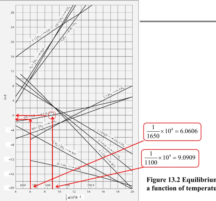
(a) the reactant consists of 1 mol of H₂O vapor and 1 mol of CO, T = 1100 K, P = 1 bar From Fig 13.2, K = 1

 

K

P

P

y

_o i v i i  

















_

_

_{ 0} i i  

 

2 2 2

1

i v _{H CO} i i _{CO H O}

y y

y

K

y y













v

n

v

n

n

n

y

i i i i

_







0 0

2

1

_e CO

y







2

2 e CO

y





2

1

2 e O H

y







2

2 e H

y





0.5

e



 

2 2 2 2 ₁ 1 1 (1 ) 2 2 e e e e e e                _{ }             From Fig 13.2, lnK = 0 or K=1. _i 1 1 1 1 0 i  



     

the reaction mixture is as an ideal gas, Eq. (13.28)

_{ }

2 2 2 1 i v _{H CO} i i CO H O y y y K y y   



Figure 13.2 Equilibrium constants as a function of temperature 4 1 10 9.0909 1100   4 1 10 6.0606 1650  × -1

-2 2 2O CO H H CO    From Fig 13.2, K = 1

 

K

P

P

y

_o i v i i  

















_

_

_{ 0} i i  

 

2 2 2

1

i v _{H CO} i i CO H O

y y

y

K

y y









(b) the same as (a) except that the pressure is 10 bar

Since v = 0, the increase in pressure has no effect on the ideal gas reaction:



_e



0

.

5

(c) the same as (a) except that 2 mol of N₂ is included in the reactants

Since N₂ does not take part in the reaction and serves as a diluent: Increasing the initial number of moles n₀ from 2 to 4.

5

.

0



e



1 4 e CO y   2 4 e CO y   2 1 4 e H O y   2 4 e H y     2 2 2 1 i v H CO i i CO H O y y y K y y   



2 2 2 2 2 4 4 ₁ 1 1 _{(1 )} 4 4 e e H CO _e e e CO H O e y y y y                              