1. INTRODUCTION
Object tracking is one of the most intriguing problems in the computer vision area. It is not only related to the problem of the shape and the color tracking of an object but also linked to that of object recognition or identification of a particular object. Recently, in the computer vision area, visual tracking of moving objects is an active research issue since the particle filter approaches [1][2][3] were proved to be efficient in object tracking especially in the cluttered environment. Particle filters are based upon the Bayesian conditional probabilities such as prior distributions and posterior ones. It is strongly believed that intelligence in robot vision would be enhanced through particle filters or the CONDENSATION(CONditional DENSity PropagATION) algorithm [3] [4] since the tracking information will eventually increase the machine intelligent quotient (MIQ) in terms of target object context, visual
planning and control. In addition to clutter, visual uncertainties such as nonlinear dynamics, non-Gaussian density, occlusion and lightness change make particle filters a necessary component in robot vision.
In this paper, we address a robust object tracking algorithm based on multiple observation models in particle filters. First of all, we choose a static webcam as the vision sensor, and assume that a human is moving in clutter. The research goal is to track a moving face or hand with the vision sensor. Now, we apply our particle filter, namely, CONDENSATION algorithm [5] to keep track of the moving face or hand. The particle filters are a class of stochastic approximations of the state posterior with a set of N weighted particles or samples
( ) ( ) 1,...,
{
i,
i}
i N
t t
X
X
= whereX
t( )i is a possible state of the thi particle at time t and
π
t( )i is the associated weight. Therefore, we perform the Monte-Carlo simulation of underlying probability distributions which may take arbitrary form, instead of deriving the analytic solution. The state( )i t
X
may be any measurable contexts such as position, velocity, rotating angle, scaling factor, tilting, etc. of a moving object. Moreover, the measureZ
tmay be any measurablequantities such as image contrast, digital image subtraction, edge-detected silhouette, 2D or 3D contours, RGB or HSV colors, etc. Each particle (contour as a particle) represents a possible state with the associated weight of a likelihood, which is measurable or computable.
In particle filters, we keep track of the state samples with the non-zero posterior probability approximated by the ensemble of the weights on all of these sampled particle sets and the idea is based upon factored sampling [6] in Bayesian inference rule described by the conditional posterior density as
1 1 1 1 1 ( ) ( ) 1 1 1 ( | ) ( | ) ( | ) = ( | ) ( | ) ( | ) ( | ) ( | ) (1) = ( | ) ( ) t t t t t t t t t t X t t t N i i t t t t t i t t t P X Z P Z X P X Z P Z X P X X P X Z P Z X P X X P Z X q X κ κ κ π κ − − − − − − − = = ≅
∫
∑
where X is the state at time t , t { ,...,1 } t
t
Z = Z Z is the observation up to time t , κ is a proportional constant,
1 ( t| t )
P X X− is the Markov-chain motion model, P Z( t|Xt) is the measurement model, and ( )1
i t
π− is the weight for particle ( ) 1 i t X− . Here, ( )1 ( )1 1 ( ) ( | ) N i i t t t t i q X π−P X X− = =
∑
is the proposaldistribution from which N samples Xt( )i are drawn by Monte-Carlo approximation of the integral. In brief, the posterior density ( 1| 1)
t t
P X− Z− is recursively approximated by the particle set { ( )1, ( )1}
i i
t t
X− π− , and then these samples are weighted by the likelihood ( )1 = P(Z |X )t-1 (i)t-1
i t
π− .
Primarily, the particle filter algorithm consists of three elementary steps: sampling, predicting, and measuring. The basic principle is the conditional probability propagation between the prior density in sampling and predicting, and the posterior density in measurement. Thus, the prior and the posterior conditional densities are calculated by taking turns in a recursive form. Existing algorithms of particle filters include CONDENSATION[4][7], Kalman particle filter (KPF) [8], and Unscented Kalman particle filter (UPF) [9]. Both KPF and UPF add the predicting models by using the state estimate with the Gaussian and non-Gaussian assumptions respectively
Visual Object Tracking based on Real-time Particle Filters
Dong- Hun Lee*, Yong-Gun Jo
**, and Hoon Kang
****
School of Electrical and Electronics Engineering, Chung-Ang University, Seoul, Korea (Tel : +82-2-816-8234; E-mail:[email protected])
**
School of Electrical and Electronics Engineering, Chung-Ang University, Seoul, Korea (Tel : +82-2-816-8234; E-mail: [email protected])
***
School of Electrical and Electronics Engineering, Chung-Ang University, Seoul, Korea (Tel : +82-2-816-8234; E-mail: [email protected])
Abstract: Particle filter is a kind of conditional density propagation model. Its similar characteristics to both selection and
mutation operator of evolutionary strategy (ES) due to its Bayesian inference rule structure, shows better performance than any other tracking algorithms. When a new object is entering the region of interest, particle filter sets which have been swarming around the existing objects have to move and track the new one instantaneously. Moreover, there is another problem that it could not track multiple objects well if they were moving away from each other after having been overlapped. To resolve reinitialization problem, we use competitive-AVQ algorithm of neural network. And we regard interfarme difference (IFD) of background images as potential field and give priority to the particles according to this IFD to track multiple objects independently. In this paper, we showed that the possibility of real-time object tracking as intelligent interfaces by simulating the deformable contour particle filters.
Keywords: Particle Filter, CONDENSATION, Active Contour, Object Tracking
This paper was performed for the intelligent robotics development program, one of the 21st century frontier R&D programs funded by the Ministry of commerce, industry and
and thus improve the tracking characteristics of the prior in terms of better proposal distributions. Three updating steps of tracking in particle filters are summarized as follows:
1) Sampling (Selection)
2) Predicting (Particle Dynamics) 3) Measuring (Output)
In the sampling phase, the importance sampling [7] incorporates hints or other sources by introducing samples at more likely spots in the state space while partitioned sampling [10] suggests that particles may be sampled hierarchically for efficiency in order to obtain equivalent results with fewer samples. Therefore, in the subsequent section, we investigate two observation models in particle filters: the point clouds of skin colors and the active contours of the B-spline snakes.
2. Particle Filters with Multiple Observation Models
for Visual Object Tracking
The CONDENSATION algorithm provides a plausible way of tracking a moving object with some features for the vision sensors in terms of a probabilistic propagation process. If the number of the object features is K, the state of the i particle th or contour becomes Xt( )i ∈ Rk , and if the particle dynamics is considered, the number of the state is increased twice as much. The basic tracking algorithm is represented as follows:
CONDENSATION Tracking Algorithm
• Given the old particle or contour set ( ) (i) 1 t-1 {Xt−i , π } , compute a new particle or contour set { ( ), t(i)}
i t
X π for i=1,… , N Initialize 0( ) = 1/N
i
π , and its cumulative distribution ( )
0 = i/N i
c .
1) Select a sample St( )i as follows:
a) Generate a uniformly distributed random numberr ∈[0,1].
b) Find the smallest
j
for which ( )1 r j t c− ≥ . c) Set ( ) = X(j)t-1 i t S .2) Predict from sampling to obtainSt( )i .
P X( t|Xt−1 t= S )(i) (2) Here, we imbed the particle dynamics by choosing one of many different equations of motion and the estimation procedure in order to find
( ) | 1 i t t S ∧
− . Note that deterministic drift and stochastic diffusion are included together by the random number generation.
3) Measure the object features and update the weights in terms of the multiple observation models
( ) (i) t t t|t-1 = P(Z |X =
S
) i t π ∧ (3) And normalize the posterior so that ( )1 = 1 N i t i π =
∑
and compute the cumulative distributionc( )ti . Update( ) (i) t
{Xti , π }. For the multiple observation models, the conjunctive or disjunctive operators may be used in order to combine the multiple object features together by using AND or OR in (P Zt|Xt) multiplication inπt( )i .
• Estimate the moments of the tracked positions or other estimates after all N particles or contours are updated as follows:
N ( ) ( ) | 1 i=1 [ ( )] = ( ) i i t t t t E g X π g
S
∧ −∑
i(4)
For the state estimate [ (E g Xt)], it is noted that there is no explicit state estimate maintained, that is, the state information is just a cloud of particle points or samples of active contours. Therefore, we may arbitrarily choose either the mean value of the particles or the confidence region of an inverse covariance matrix. Moreover, one element of the state, for example, the average position of the target object is estimated for updating the next position of the target object centroid.
2.1 Sampling (Selection)
In the sampling stage, we select N particle samples by picking them randomly and uniformly in [0,1] from the normalized weights given by ( )
1 = 1 N i t i π =
∑
. This selection approach is the same as the roulette-wheel selection as in the genetic algorithm (GA), which is equivalent to spinning a roulette wheel with the arc-lengths of bins equal to the particle weights. Then, the particles are resampled according to the score, that is, highly likely particles are duplicated while unlikely ones are eliminated. This results in adaptive focusing on more promising areas of the state space.2.2 Prediction (Particle dynamics)
The prediction step is to place each particle or contour from the generative form of dynamics given by
( ) (i) t-1 t-1 = f(S ) + i t S ε (5) Where f() is a deterministic component and εt is a random component. Usually, f() represents a nonlinear drift of each particle with different displacement and εt is an independent diffusion of each particle typically modeled with a white noise. Therefore, we often use the extended Kalman filters (EKF) as the prediction model in order to estimate
( ) | 1 i t t
S
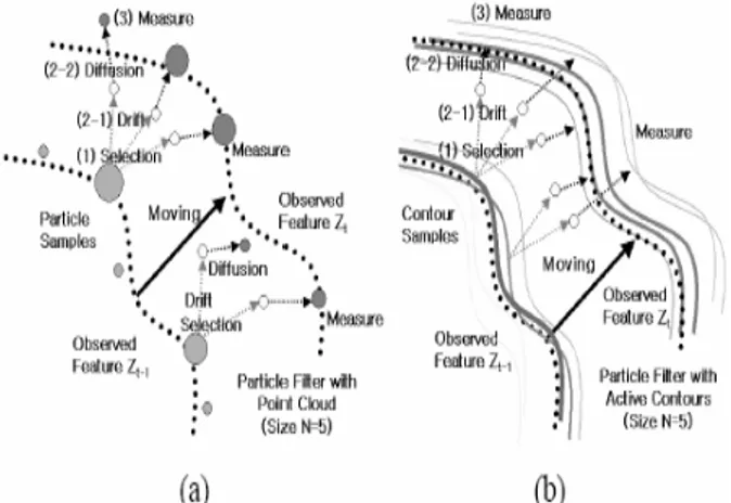
∧ − by assumingthat noise characteristics complies with Gaussian. The particle or contour dynamics is related to the observation model in such a way that it might lead to the features of higher likelihood observation as shown in Figure 1.
Figure 1. Observation Mechanisms in the Predicting and the Measuring Stages: (a) 5 Particle Samples of Point Cloud and (b) 5 Particle Samples of Deformable Contours
2.3 Measurement (Output)
For each particle or contourXt( )i , we compute new weight ( )i
t
π using the measurement likelihood ( ) (i) t t = P(Z |X ) i t π (6) and find the plausibility conditions such that the particles with impossible configurations are given zero likelihood. For example, the positions outside of the image features of interest are givenπt( )i = 0
.
2.4 Multiple Observation Models
In this paper, we choose two object features for face or hand tracking. One is the contrast information from the digitally subtracted images and the other is the skin-color information from the HSV color model. The former measure of the subtracted images ∆ is defined by Pt
t t-( , ) = |I t-(x,y) - I (x,y) | t P x y ∆ ∆ (7) where I x y is the ( , )t( , ) th
x y pixel value of the image at time t in [0,1] and It−∆ is the delayed image at time frame t− ∆ . Also, the latter measure of the skin color is based on the HSV model where the hue and the saturation information are used by computing the Gaussian density function
2 2 R 2 -(h(x,y)-h (x,y)) ( ( , ) ( , )) ( , ) = exp( ) 2 R t hs s x y s x y C x y σ − − (8)
Whereσhs is the equivalent standard deviation for the HS features;
( , ) t
C x y is the ( , )x yth feature of the skin color; ( , )h x y and ( , )
s x y are the hue and the saturation values of a color-measured control point at (x,y), and hR( , )x y and
( , ) R
s x y are the hue and the saturation references for the initial particle subset, respectively. Now we consider the observation models for the convectional particle sets of point cloud and for the deformable contours [5] of the B-spline snakes.
• Point Cloud as Particles:
- For the ith particle's point (xp,yp)∈ ∆ of both the Pi subtracted pixel and the associated skin-color point, the weight of the prior is computed by using the disjunctive operator (OR): P P i ( ) P P t P P (x ,y ) P = { (x ,y ) + C (x ,y )} i t t w P λ ∈∆ ∆
∑
(9)- The state vector for one particle is defined as ( )
[ ( ), ( ), ( 1), ( 1)]
i T
t P P P P
X = x t y t x t− y t− at time t and the dynamics is represented by
t-1
AX t
t v
X = +B (10) where A, B are the appropriate matrices, and v is the white t noise with diffusion covariance matrix about the two axes. • Deformable Contours as Particles:
- For the control points of the i contour, (th xP,yP)∈ of Pi the subtracted image, and for the corresponding i th skin-color control points (xC,yC)∈Ci , the weight of the prior is computed by using the conjunctive operator (AND):
i i ( ) ( ,y ) P ( ,y ) = ( , ) ( ,y ) P P C C i t t P P t C C x x C w P x y λC x ∈∆ ∆ ∈
∑
∑
(11)- The state vector for one particle is defined as
( ) T P P P P = [x (t), (t), (t), (t),x (t-1), (t-1), (t-1), (t-1)] i t X y θ α y θ α is
the centroid of the control points in ∆Pi; , θ α are the rotating angle and the scaling factor of the B-spline snake, respectively; and the dynamics is similarly described by (10).
Note that λ is the balancing coefficient between two independent object features as the conjunctive or disjunctive operators are used for them. Also, the posterior πtis obtained by resampling and normalization such as
N
= f [ ( ( ))] t fR fN wt
π (12) where, ,fN f are the normalization and the resampling R functions, respectively, and w is given in (9) and (11). The t deformable contour of the i particle has the form of the th planar affine shape space as
t x y y T P P ' WY 1 0 Q 0 0 Q = 0 1 0 Q Q 0
= [x , ,cos 1 ,cos 1 ,sin ,sin ] x t Q Q W Y y θ α θ α θ θ = + ⎡ ⎤ ⎢ ⎥ ⎢ ⎥ ⎣ ⎦ − + − + (13)
where W is the shape matrix, Y is the shape-space vector t computed from X , and t
T T T x y ', = [Q ,Q ]
Q Q are the updated and the reference control point vector, respectively. Here, the updated control point vector Q is represented by '
T
P,1 P,n P,1 P,n
' = [x (t),...,x (t);y (t),...,y (t)]
Q (14)
where n is the total number of the control points in a B-spline snake.
3. Experimental Results of Visual Object
Tracking with Particle Filters
Now three cases of the multiple observation models are applied to visual object (face or hand) tracking based on the particle filters in the experiment.
3.1 Robust Face Tracking Based On Particle Filters
of Point Cloud
For the simulation of face tracking with a particle cloud, we choose the number of particles, 50 N = and the particle observation model, (9) in order to combine both the contrast and the skin-color features together. Here, λ = 1/N , and the threshold of π( )i for the effective particle size is 2/ N for adaptive resampling. The standard deviations for diffusion in both axes are σx= σy = 30 and those for the hue and the saturation are selected as σhs = 0.05. Figure 2 shows visual face tracking with particle filters of point cloud using both subtracted images and skin colors.
Figure 2. Experiment of Visual Face Tracking with Particle Filters of Point Cloud using Both Subtracted Images and Skin Colors (N=50)
Figure 3. Experiment of Visual Hand Tracking with Deformable Contours using Subtracted Images Only
Figure 4. Experiment of Visual Face Tracking with Deformable Contours using Both Subtracted Images and Skin Colors (N=100)
Figure 5. Experiment of Visual Face Tracking with Deformable Contours using Both Subtracted Images and Skin Colors (N=50)
3.2 Robust Hand Tracking Based On Deformable
Active Contours
For the simulation of hand tracking with contours, we choose the number of particles, 200 N =200 and the deformable observation model, (9). But, in this case, we take only the contrast features into account by setting λ= , the number 0 of control points in the B-spline snake is n=45 , and the threshold of π ( )i for the effective particle size is 1.5/ N during adaptive resampling. The standard deviations for diffusion in both axes are σx=σy= and those for the 5 rotating angle and the scaling factor are selected as
3(deg.), 0.05
θ α
σ = σ = , respectively. In Figure 3, it is demonstrated that visual hand tracking is performed with the B-spline snake of deformable contours using subtracted images only.
3.3 Robust Face Tracking Based On Deformable
Active Contours and Skin-Colors
Finally, for the simulation of human face tracking with both point clouds and contours, we choose the number of particles, N=50 or N=100 and the observation model, (11) in order to combine both the contrast and the skin-color features together.
Here, the number of control points is n=21 and the threshold of π ( )i for the effective particle size is 1.5/ N for adaptive resampling. The standard deviations for diffusion in both axes are 5σx=σy= , those for the rotating angle and the scaling factor are selected as σθ=1(deg.),σα=0.01 , respectively, and those for the hue and the saturation are selected as
0.05 hs
σ = . However, by using the multiple observation models (λ=1/N) such as deformable contours and a constrained point cloud of both subtracted images and skin colors under the same conditions, we could significantly reduce the number of particle sets in the above cases by half with better tracking results as shown in Figures 4 and 5, respectively.
4. Competitive-AVQ for Reinitialization Procedure
Particle filter of point cloud can be realized in real-time. However, particle filter has inherent problem which is initialization point. When a new object is detected somewhere part of interface, particle filter Set in pause position has to move and tracking the new object instantaneously. In order to do that, we use competitive-AVQ algorithm of neural network. This algorithm defines an area which made stripe of image plane boundary. And it is used when IFD data exceeds a threshold value of stripe area. The c-AVQ algorithm is represented as follows:
c-AVQ for PF Reinitialization
- Check boundary stripes PB with threshold (3%~4% IFD data), if the condition holds,
- For all pt(k) in PB > threshold at time t, find the winner (the ith cluster)
{
}
*
2
( ) arg min ( ) ( ) #(cluster)
i j j t w k = ⋅ w k −p k j→
(
)
* * * B ( 1) ( ) ( ) ( ) #(P ) i i t i w k+ =w k +µ
p k −w k k→- Update the ith particle state s.t. the average is shifted to the ith cluster center (the winner)
* i
t i
5. Priority-based Subtraction of Background
IFD & Effective Particle Size
Multiple object tracking regards interframe difference (IFD) as potential field (V). After regarding that, it determines the priority for many particles and repeats a sampling (selection), particle dynamic, output one by one how to subtract with priority at IFD buffer. This subtraction method is like subtractive clustering algorithm. If this method is used, object tracking can be done at different direction though two objects cross each other.
0 K k-1 V = P V = P-V , k = 1~# (PF Set) ∆ ∆ (15) When several measurement values or a uniform posterior distribution is appeared, effective particle size,Neff, is used in resampling stage and is defined as follows:
N 2 i i=1 = 1/( ) eff N
∑
π (16) Therefore, if Neff is very small or large, resampling is attempted. In this case will be happen when the object is paused and when the tracking is failed. Figure 6 shows experiment result using real-time multiple object tracking based on point cloud method.
6. Conclusions and Discussion
In this paper, the CONDENSATION algorithm is extended to combining the multiple observation models such as particle clouds, contour tracking, digital subtraction and skin color, with application to human face or hand tracking, where multiple object features are measured with the prior and posterior probability densities are propagated in order to obtain the state estimates such as the target average position, the angles of principal axis, the scaling factors, etc. From the experimental results, the suggested particle filters with multiple observation models demonstrated robust visual tracking in uncertainties such as clutter and nonlinear motion.
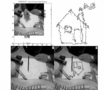
The advantages of particle filters with multiple observation models are demonstrated here with application to face or hand tracking in robot vision. First, the particle filters can have target object dynamics embedded easily by combining nonlinear dynamics and multiple observation models with a smaller particle size. Second, Clutter in the measurement likelihood that causes the multi-modal posterior can be dealt with robustly. Third, point clouds, control points, and statistical parameters in particle or contour tracking may be simply converted to the image segmentation. And finally, it is possible to apply particle filters to high-level inference of context semantics by using the 2D or 3D contour information as shown in Figure 7 where the tracking result of picture drawing is demonstrated. For the future works, we will investigate the multiple object particle filters as well as the real-time implementation of particle filters for contour tracking.
Figure 6. Real-time particle filter for multiple objects
Figure 7. Picture Drawing Results with Particle Filters of Multiple Observation Models (N=200)
REFERENCES
[1] J.M. Hammersley and K.W. Morton, “Poor man's monte carlo,” J. of the Royal Statistical Society B, vol. 16, pp.23-38, 1954.
[2] N. Gordon, D. Salmond, and A. Smith, “Novel approach to nonlinear/non-gaussian bayesian state estimation,” IEEE Proc. F, vol. 140, no.2, pp. 107-113, 1993.
[3] M. Isard and A. Blake, “Contour tracking by stochastic propagation of conditional density,” in Proc. 4th European Conf. on Computer Vision (ECCV), pp. 343-356, April 1996 [4] M. Isard and A. Blake, “Condensation-conditional density propagation for visual tracking,” Int. J. Computer Vision, vol 29, no. 1, pp. 5-28, 1998.
[5] A. Blake and M. Isard, Active Contours, London: SpringerVerlag, 1998.
[6] A. Popoulis, Probability and Statistics, New York: PrenticeHall, Inc., 1990.
[7] M. Isard and A. Blake, “Icondensation: Unifying low-level and high-level tracking in a stochastic framework,” in Proc. 5th European Conf. on Computer Vision (ECCV), pp. 893-908, April 1998.
[8] A. Blake, M. Isard, and D. Reynard, “Learning to track the visual motion of contours,” J. Artificial Intelligence, vol 78, pp. 101-134, 1995.
[9] S.J. Julier and J.K. Uhlmann, “A new extension of kalman filter to linear system,” in Proc. Aerosense: 11th Int. Symp. On Aerospace/Defense Sensing, Simulation, and Control, Orlando, FL, pp. 182-193, 1997.
[10] J.M. Jurada, Introduction to Artificial Neural Systems, New York: West Pub.Co., 1992
[11] R. Malladi, J. A. Sethian and B. C. Vemuri, “Shape Modeling with Front Propagation: A Level Set Approach”, IEEE Trans. On Pattern Analysis and Machine Intelligence, vol.17,no. 2,pp.158-175,Feb.1995
[12] J. MacCormick and A. Blake, “Partitioned sampling, articulated objects and interface-quality hand tracking,” in Proc. 7th European Conf. on Computer Vision (ECCV), April 2000.
[13] Freedman, D and Tao Zhang "Active contours for tracking distributions", IEEE Trans. on Image Processing, vol. 13, no. 4, PP. 518 - 526, 2004.
[14] C. Gentile, O. Camps and M. Sznaier, "Segmentation for robust tracking in the presence of severe occlusion", IEEE Trans. on Image Processing, vol. 13, no. 2, pp. 166 - 178, 2004.
[15] F. Gustafsson, F. Gunnarsson, N. Bergman, U. Forssell, J. Jansson, R. Karlsson and P.-J. Nordlund, "Particle filters for positioning, navigation, and tracking", IEEE Trans. on Signal Processing, vol. 50, no. 2, pp. 425 - 437, Feb. 2002.
[16] C. Hue, J.-P. Le Cadre and P. Perez, "Tracking multiple objects with particle filtering", IEEE Trans. on Aerospace and Electronic Systems, vol. 38, no. 3, pp. 791 - 812, 2002.