Analysis of Kinematic Mapping Between an Exoskeleton Master Robot and a Human Like Slave Robot With Two Arms

1. INTRODUCTION

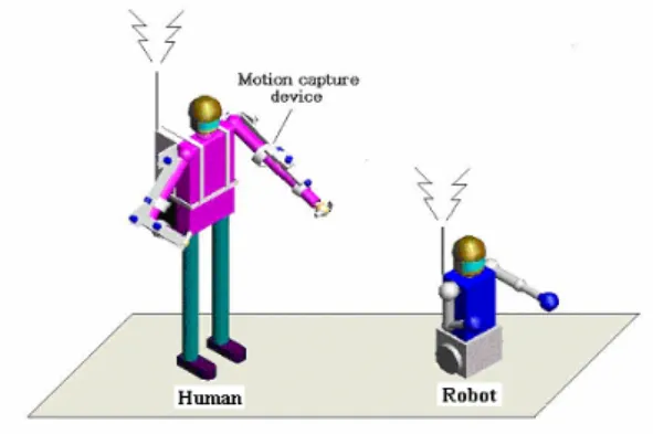
Recently, interaction between robots and humans has been enormously increased in a variety of types as the technology of service robots are developed further [1-4]. There are many representing types of interaction between robots and human operators. Robot pets are a good interactive example of exchanging emotions. One simple interaction with robots is a tele-operated control [5-7]. Using a joystick, an operator can control the movement of the slave robot with visual feedback of movement. A human operator controls remotely located robots. Here one basic requirement of the salve robot is the accurate motion following after the master. This requires an accurate mapping.

For a motion following task, the slave robot is required to follow after the movement of the master robot exactly. The operator wears the exoskeleton robot to generate motions, then the slave robot is required to follow the motion after the motion of the master robot.

To synchronize motions of two robots, position control by kinematic analysis of mapping is required since two robots are designed slightly in different configuration. The exoskeleton robot is not actuated by motors so that it has a more flexible structure in design. However, the two arm robot is actually actuated by motors commanded from the exoskeleton by wireless communication. It has to allow housings for motors. So there is a slightly different configuration between two robots. This different kinematic configuration leads to asynchronous movements in the Cartesian coordinates. To synchronize movements, kinematic analysis is required to compensate for mismatched parameters.

In this paper, kinematic analysis of two robots is presented and compared. Forward kinematics and inverse kinematics are found. Movement of the exoskeleton master robot is captured by encoders. Those encoder data are converted to joint angle values and those values are used to calculate end-effector positions. Those end-effector positions are used to calculate inverse kinematic solutions of the slave robot to generate desired joint values. Then the controller of the slave robot actuates and moves the arms. Encoder values of the slave robot are also used for calculating position of the end-effector through forward kinematics. Two end-effector position values are compared. This confirms the synchronous kinematic mapping.

In this framework, to do that, inverse kinematics solutions

of the slave robot are found. Simulation studies are conducted to confirm that kinematic analysis is correct. Experiments are also conducted to confirm the feasibility of the analysis.

Fig 1. Concept of motion following robot

2. OVERALL STRUCTURE

2.1 The exoskeleton master robot

Fig.2 shows the exoskeleton master robot. It has the total 12 d.o.fs. It is designed for the human operator to wear to move arms. Movements are captured by joint encoders.

Fig 2. Motion capture exoskeleton master robot.

Analysis of Kinematic Mapping Between an Exoskeleton Master Robot and a Human Like Slave

Robot With Two Arms

Deok Hee Song*, Woon Kyu Lee**, and Seul Jung***

* Department of Mechatronics Engineering, Chungnam National University, Daejeon, Korea (Tel : +82-42-821-6876; E-mail: {*[email protected],**[email protected], ***[email protected]})

Abstract:

This paper presents the kinematic analysis of two robots, an exoskeleton type master robot and a human like slave robot with two arms. Two robots are designed and built to be equivalent as motion following robots. The operator wears the exoskeleton robot to generate motions, then the slave robot is required to follow after the motion of the master robot. However, different kinematic configuration yields position mismatches of the end-effectors. To synchronize motions of two robots, kinematic analysis of mapping is analyzed. The forward and inverse kinematics have been simulated and the corresponding experiments are also conducted to confirm the proposed mapping analysis.

2.2 The human like slave robot

The slave robot has two arms as shown in Fig.3.

Fig 3. The slave robot with two arms

The slave robot also has 12 d.o.fs. Each joint of the slave robot is actuated.

3. KINEMATICS ANALYSIS

3.1 Forward kinematics

Fig. 4 and Fig. 5 show the coordinate transforms of the master robot and the slave robot, respectively [8].

Fig . 4. Coordinate representation of the exoskeleton master robot. 1 θ 2 θ 3 θ 4 θ 5 θ θ6

Fig 5. Coordinate representation of the slave robot Table 1 lists D-H parameters for the master robot Table 1. D-H parameters & Joint range of the master robot

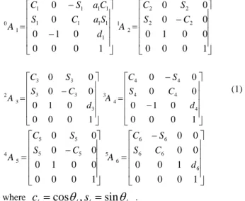
From D-H parameters, transformation matrices are obtained.

⎥ ⎥ ⎥ ⎥ ⎦ ⎤ ⎢ ⎢ ⎢ ⎢ ⎣ ⎡ − = ⎥ ⎥ ⎥ ⎥ ⎦ ⎤ ⎢ ⎢ ⎢ ⎢ ⎣ ⎡ − − = 1 0 0 0 0 0 1 0 0 0 0 0 1 0 0 0 0 1 0 0 0 2 2 2 2 2 1 1 1 1 1 1 1 1 1 1 1 0 S C S C A d S a C S C a S C A ⎥ ⎥ ⎥ ⎥ ⎦ ⎤ ⎢ ⎢ ⎢ ⎢ ⎣ ⎡ − − = ⎥ ⎥ ⎥ ⎥ ⎦ ⎤ ⎢ ⎢ ⎢ ⎢ ⎣ ⎡ − = 1 0 0 0 0 1 0 0 0 0 0 1 0 0 0 0 1 0 0 0 0 0 4 4 4 4 4 4 3 3 3 3 3 3 3 2 d C S S C A d C S S C A (1) ⎥ ⎥ ⎥ ⎥ ⎦ ⎤ ⎢ ⎢ ⎢ ⎢ ⎣ ⎡ − = ⎥ ⎥ ⎥ ⎥ ⎦ ⎤ ⎢ ⎢ ⎢ ⎢ ⎣ ⎡ − = 1 0 0 0 1 0 0 0 0 0 0 1 0 0 0 0 0 1 0 0 0 0 0 6 6 6 6 6 6 5 5 5 5 5 5 4 d C S S C A C S S C A

where

c

_i

=

cos

θ

_i

,

s

_i

=

sin

θ

_i .

Table 2 shows the D-H parameters of the slave robot. Table 2. D-H parameters & Joint range of the slave robot

Joint

θ

_i

α

_i

a

_i

d

_i Joint range

(degree) 1 0 -90

a

₁

d

₁ -45 to 45 2 90 90 0 0 -90 to 90 3 90 90 0

d

₃ 80 to 270 4 0 -90 0

d

₄ -90 to 90 5 90 90 0 0 0 to 160 6 0 0 0

d

₆ -90 to 90

Joint

θ

_i

α

_i

a

_i

d

_i Joint range (degree) 1 90 90 0 0 45 to 45 2 90 90 0

d

₂ 80 to 270 3 90 -90 0 0 0 to 90 4 -90 -90 0

d

₄ -180 to 0 5 90 90 0 0 0 to 160 6 0 0 0

d

₆ -90 to 90

We see from two tables that configurations of Joint 1 to joint 3 are different and the rest of joint configuration are same. This different configuration causes different movements in the end-effector position. The goal is to align the movement of two robots. The corresponding transformation matrices are shown in (2). ⎥ ⎥ ⎥ ⎥ ⎦ ⎤ ⎢ ⎢ ⎢ ⎢ ⎣ ⎡ − = ⎥ ⎥ ⎥ ⎥ ⎦ ⎤ ⎢ ⎢ ⎢ ⎢ ⎣ ⎡ − = ⎥ ⎥ ⎥ ⎥ ⎦ ⎤ ⎢ ⎢ ⎢ ⎢ ⎣ ⎡ − − = ⎥ ⎥ ⎥ ⎥ ⎦ ⎤ ⎢ ⎢ ⎢ ⎢ ⎣ ⎡ − − = ⎥ ⎥ ⎥ ⎥ ⎦ ⎤ ⎢ ⎢ ⎢ ⎢ ⎣ ⎡ − = ⎥ ⎥ ⎥ ⎥ ⎦ ⎤ ⎢ ⎢ ⎢ ⎢ ⎣ ⎡ − = 1 0 0 0 6 1 0 0 0 0 0 0 1 0 0 0 0 0 1 0 0 0 0 0 1 0 0 0 4 0 1 0 0 0 0 0 1 0 0 0 0 0 1 0 0 0 0 0 1 0 0 0 2 0 1 0 0 0 0 0 1 0 0 0 0 0 1 0 0 0 0 0 6 6 6 6 6 5 5 5 5 5 5 4 4 4 4 4 4 3 3 3 3 3 3 2 2 2 2 2 2 1 1 1 1 1 1 0 d C S S C A C S S C A d C S S C A C S S C A d C S S C A C S S C A (2)

The end-effector position can be obtained from the following matrix.

⎥

⎥

⎥

⎥

⎦

⎤

⎢

⎢

⎢

⎢

⎣

⎡

=

=

1

0

0

0

6 0 6 0 z z z z y y y y x x x x

p

a

s

n

p

a

s

n

p

a

s

n

A

T

(3) 3.2 Inverse kinematics

1) Inverse kinematics of the master robot From Fig. 4,

P

₅ is given as

⎥

⎥

⎥

⎦

⎤

⎢

⎢

⎢

⎣

⎡

+

+

−

−

+

+

+

+

+

+

=

−

=

1 2 3 3 2 4 1 3 4 1 1 2 3 3 2 4 1 3 4 1 1 2 3 3 2 4 6 6 5

)

(

)

(

)

(

)

(

d

C

d

S

S

d

C

C

d

S

a

S

d

S

C

d

S

C

d

C

a

S

d

S

C

d

a

d

p

p

(4) where

a

=

[

a

_x

a

_y

a

_z

]

T.

Solutions of

θ

₁

,

θ

₂

,

θ

₃are analyzed as two cases of

0

2

=

θ

and

θ

2

≠

0

depending upon the value of

sin

θ

2.

The corresponding results are as follows:

i) [

θ

2

=

0

]

]

[

tan

2 5 2 2 5 2 5 2 2 5 1 1 x x x x

p

B

A

B

Ap

p

B

A

A

Bp

−

+

±

−

−

+

±

=

−

θ

(5)

0

2

=

θ

(6)

]

2

[

sin

1 3

D

E

−

=

−

θ

(7) ii)[

θ

₂

≠

0

]

]

[

tan

2 5 2 2 5 2 5 2 2 5 1 1 x x x x

p

B

A

B

Ap

p

B

A

A

Bp

−

+

±

−

−

+

±

=

−

θ

(8)

]

[

tan

2 2 2 2 2 2 1 2

F

H

G

H

FG

F

H

G

G

FH

−

+

±

−

−

+

±

=

−

θ

(9)

]

)

(

1

[

tan

2 5 1 2 3 5 1 2 3 1 3 z z

p

d

C

d

p

d

C

d

−

+

−

−

+

±

=

−

θ

(10) where 2 1 2 5 1 2 3 2 4 2 5 2 5 5 1 1 1 3 2 5 2 5 2 4 2 1 1 2 4 3 4 1 2 3 3 2 4 ) ( ) ( 2 , 2 , , , a p d d d p p H p d a G a d F p p d a E a C d D C d B a S d S C d A z y x z y x − − + − − + ≡ − ≡ ≡ − − + ≡ ≡ ≡ + + ≡ .

Solutions for

θ

₄

,

θ

₅

,

θ

₆are given as ] [ tan1 4 J I − =

θ

(11) ] [ tan1 5 L K − = θ (12) ] [ tan1 6 N M − = θ (13) where z y x z y x z y x z y x z y x z y x s C C S C S s C S S S S C C C S s C S C S S S C C C N n C C S C S n C S S S S C C C S n C S C S S S C C C M a S S a C C S C S a C S S C C L a S C C C S a S S S C S C C C S a S S C C S S C C C K a C S a S C C C S a S S C C C J a C a S S a S C I ) ( ] ) ( [ ] ) ( [ ) ( ] ) ( [ ] ) ( [ ) ( ) ( ) ( ] ) [( ] ) [( ) ( ) ( 4 2 4 3 2 4 2 1 4 3 1 3 2 1 4 2 1 4 3 1 3 2 1 4 2 4 3 2 4 2 1 4 3 1 3 2 1 4 2 1 4 3 1 3 2 1 3 2 3 1 3 2 1 3 1 3 2 1 4 2 4 3 2 4 2 1 4 3 1 3 2 1 4 2 1 4 3 1 3 2 1 3 2 3 1 3 2 1 3 1 3 2 1 2 2 1 2 1 + + + + − + + − − ≡ + + + + − + + − − ≡ − − + + ≡ + − + + + + + − ≡ − + + − ≡ + + ≡

2) Inverse kinematics of the slave robot i)

θ

₁

,

θ

₂

,

θ

₃ ⎥ ⎥ ⎥ ⎦ ⎤ ⎢ ⎢ ⎢ ⎣ ⎡ − − + − + − = = − = 3 2 4 1 2 3 2 1 3 1 4 1 2 3 2 1 3 1 4 6 6 ) ( ) ( ) , , ( S S d C d S C S C C d S d S C C C S d p p p a d p p T z y x (14) where

a

=

[

a

_x

,

a

_y

,

a

_z

]

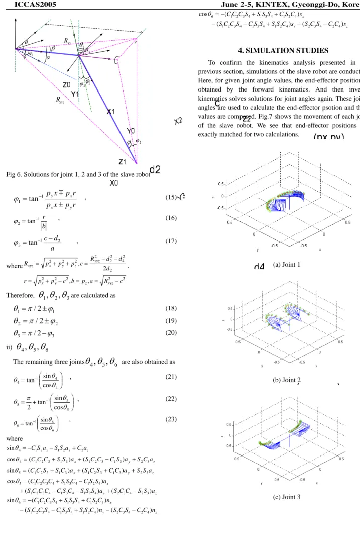
T.

2 θ 3 θ 1 θ φ α β 1 ϕ 2 ϕ 2 ϕ 3 ϕ 3 ϕ xyz R xy R

Fig 6. Solutions for joint 1, 2 and 3 of the slave robot

r

p

x

p

r

p

x

p

y x x y

±

=

−1

m

1

tan

ϕ

, (15) b r 1 2 tan − = ϕ , (16) a d c ₂ 1 3 tan − = −

ϕ

, (17) where 2 2 2 2 2 2 2 4 2 2 2 2 2 2 , , 2 , c R a p b c p p r d d d R c p p p R xyz z y x xyz z y x xyz − = = − + = − + = + + = _.

Therefore,

θ

₁

,

θ

₂

,

θ

₃are calculated as

1 1

π

/

2

ϕ

θ

=

±

(18) 2 2

π

/

2

ϕ

θ

=

±

(19) 3 3

π

/

2

ϕ

θ

=

−

(20) ii)

θ

₄

,

θ

₅

,

θ

₆

The remaining three joints

θ

₄

,

θ

₅

,

θ

₆ are also obtained as ⎟⎟ ⎠ ⎞ ⎜⎜ ⎝ ⎛ = − 4 4 1 4 cos sin tan θ θ θ , (21) ⎟⎟ ⎠ ⎞ ⎜⎜ ⎝ ⎛ + = − 5 5 1 5 cos sin tan 2 θ θ π θ , (22) ⎟⎟ ⎠ ⎞ ⎜⎜ ⎝ ⎛ = − 6 6 1 6 cos sin tan θ θ θ , (23) where z y x SSa Ca a S C_{1 2 1 2 2} 4 sinθ =− − + z y x SCC CS a S Ca a S S C C C1 2 3 1 3 1 2 3 1 3 2 3 4 ( ) ( ) cosθ = + + − + z y x SC S CC a S S a a C S S C C_{1 2 3 1 3 1 2 3 1 3 2 3} 5 ( ) ( ) sinθ = − + + + z y x a S S C C S a S S S C S C C C C S a S S C C S S C C C C ) ( ) ( ) ( cos 3 2 4 3 2 4 2 1 4 3 1 4 3 2 1 4 2 1 4 3 1 4 3 2 1 5 − + − − + − + = θ z y x n C C S C S n C S S S S C S C C S n C S C S S S S C C C ) ( ) ( ) ( sin 4 2 4 3 2 4 2 1 4 3 1 4 3 2 1 4 2 1 4 3 1 4 3 2 1 6 − − + − − + + − = θ z y x s C C S C S s C S S S S C S C C S s C S C S S S S C C C ) ( ) ( ) ( cos 4 2 4 3 2 4 2 1 4 3 1 4 3 2 1 4 2 1 4 3 1 4 3 2 1 6 − − + − − + + − = θ

4. SIMULATION STUDIES

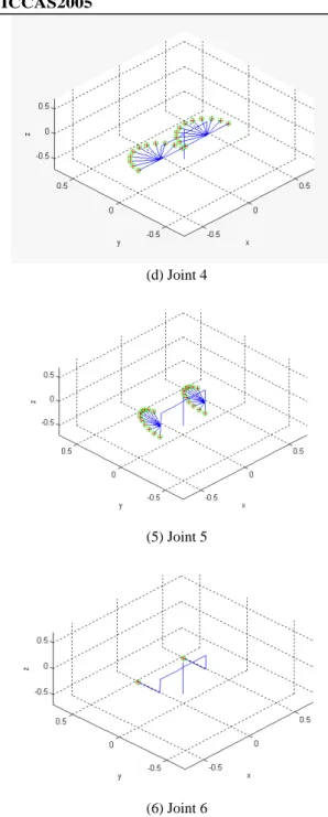
To confirm the kinematics analysis presented in the previous section, simulations of the slave robot are conducted. Here, for given joint angle values, the end-effector position is obtained by the forward kinematics. And then inverse kinematics solves solutions for joint angles again. These joints angles are used to calculate the end-effector psotion and their values are compared. Fig.7 shows the movement of each joint of the slave robot. We see that end-effector positions are exactly matched for two calculations.

(a) Joint 1

(b) Joint 2

(d) Joint 4

(5) Joint 5

(6) Joint 6

Fig 7. Simulation results of inverse kinematics of the slave robot

Fig 8. Movements of all joints

Fig.8 shows the movement of all of the joints of the slave robot. We see that the end-effector position exactly matched. This simulation confirms that the kinematic analysis of the slave robot is correct. Simulation for the master robot does not appear here since it has been already presented in our previous research [8].

5. MAPPING BETWEEN TWO ROBOTS

5.1 Kinematic mapping

Table 3 shows the D-H parameters of two robots. We clearly see that joint 1 through joint 3 are different from two robots. Different rotating frame yields different D-H parameters as well as different length of the arm.

Table 3. Comparison of D-H parameters of two robots

Exoskeleton(m) Robot manipulator (m)

Link i

a

d

_i

a

_i

d

_i 1 0.1 0.05 0 0 2 0 0 0 0.16 3 0 0.15 0 0 4 0 0.4 0 0.275 5 0 0 0 0 6 0 0.4 0 0.25 Since the workspace of the slave robot is slightly smaller than that of the master robot, we should find the factor that scales the movement in the Cartesian space. We have followed the next procedure:

1. First, the two base coordinates are aligned together by moving z axis of the master robot by the length of d₁

2. Second, the ratio of the link length is found. We have found values of a scaling factor as 0.64, 0.6875, 0.625 for each axis.

These values are obtained by comparing each link length. These factors are multiplied to the Cartesian position of the exoskeleton robot after obtaining the transformation matrix

6 0

A

T

=

. 5.1 Experiment 1. Wi

thout mapping

(b) Positional mismatching errors Fig 9 Experiment 1 : Without mapping

5.3 Experiment 2 : with scaling factor

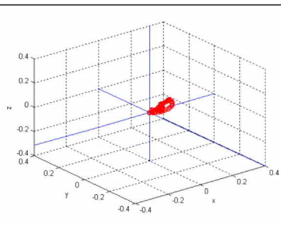
Fig 10 shows the movement of two robots. Encoder data from the master robot are obtained first. These data are used to calculate the end-effector position of the master robot. Then scale it down by the factor. These scaled down values are used to calculate joint values of the slave robot by the inverse kinematics. Then the end-effector position of the slave robot is calculated and plotted in Fig. 10.

(a) End-effector positions of two robots

(b) Positional mismatching errors Fig 10. Experiment 2:with mapping

Define abbreviations and acronyms the first time they are used in the text, even after they have been defined in the

abstract.

5. CONCLUSIONS

This paper presented kinematics mapping between two robots: the master and the slave. Two robots have different configurations due to the difficulty of implementation to represent the same position. This problem has been solved by solving inverse kinematics solution of the slave robot and by finding the scaling factor of coordinate transform. Even though the scaling factor was found to be constant in this case, mapping errors are small with acceptable ranges.

In the future, successive movements of two robots will be tested.

ACKNOWLEDGMENTS

This research has been supported by the contract of KOSEF/KRF 05-2003-000-10389-0 in Korea.

.

REFERENCES

[1] Sokho Chang, Jungtae Kim, Jin Hwan Borm, Chongwon Lee, and Jong Ok Park, “Kist teleoperation system for humanoid robot”, IEEE/RSJ Conf. on Intelligent Robots

and Systems, vol. Ⅱ, pp. 1198-12-3, 1999.

[2] M. Oda, T.Doi, and K. Wakata, “Tele-manipulation of a satellite mounted robot by an on-ground astronaut”, IEEE

Conf. on Robotics and Automations, pp. 1891-1896, 2001. [3] J. Funda, R. H. Taylor, S. Gomory, and K. G. Gruben,

“Constrained catesian motion control for teleoperated surgical robots”, IEEE trans. on Robotics and Automations, vol. 12, pp. 453-465, 1996.

[4] T. Mori, K. Tsujioka, and T. Sato, "Human-like Action Recognition System on Whole Body Motion-captured File"

IEEE Conf. on International Conference on Intelligent Robots and Systems, pp. 2066-2073, Hawaii, USA, 2001. [5] S. Jung, P. W. Jeon ,and H. T. Cho, "Interface Between

Robot and Human: Application to Boxing Robot"

International Federation of Automatic Control, 2002. [6] P. W. Jeon, P. S. Jang, B. K. Ju, K. H. Cho, and S. Jung,

“Development of boxing robot system for mechatronics education”, Korean Automatic Control Conference(in

korea), 2000.

[7] K. S. Fu, R. C. Gonzalez, and C. S. G. Lee, "ROBOTICS :

Control, Sensing, Vision, and Intelligence" McGraw-Hill, 1987.T. A. Lasky and B. Ravani, “Sensor based path Planning and Motion Control for a Robotic System for Roadway Crack Tracking”, pp. 609-622, IEEE Trans. On

Control Systems Technology, col. 8, No. 4, 2000

[8] Poong Woo Jeon & Seul Jung, “Teleoperated Control of Mobile Robot Using Exoskeleton Type Motion Capturing Device Through Wireless Communication”, IEEE/ASME