A NUMERICAL ANALYSIS OF THE WAVE FORCES ON VERTICAL CYLINDERS BY BOUNDARY ELEMENT METHOD

A MASTER’S THESIS

A NUMERICAL ANALYSIS OF THE WAVE

FORCES ON VERTICAL CYLINDERS BY

BOUNDARY ELEMENT METHOD

CHEJU NATIONAL UNIVERSITY GRADUATE SCHOOL

Department of Civil & Ocean Engineering

Cao Tan Ngoc Than

A NUMERICAL ANALYSIS OF THE WAVE

FORCES ON VERTICAL CYLINDERS BY

BOUNDARY ELEMENT METHOD

Cao Tan Ngoc Than

(Supervised by Professor Nam-Hyeong Kim)

A thesis submitted in partial fulfillment of the requirement for the

Degree of Master of Engineering

2009.2

This thesis has been examined and approved

Thesis director, Sang-Jin Kim, Prof. of Civil & Ocean Engineering

Thesis director, Byoung-Gul Lee, Prof. of Civil & Ocean Engineering

Thesis director, Nam-Hyeong Kim, Prof. of Civil & Ocean Engineering

February.2009

Department of Civil & Ocean Engineering

GRADUATE SCHOOL

CONTENTS

Contents ... ..i List of Figures...iii Summary... …viii CHAPTER 1: INTRODUCTION ... .1 1.1 Background ... .1 1.2 Objectives ... .2 1.3 Study contents... …...3

CHAPTER 2: FORMULATION OF BOUNDARY ELEMENT ANALYSIS ... .5

2.1 Diffraction phenomenon ... .5

2.2 Basic equations and boundary conditions... .8

2.3 Green function ... ..12

2.4 Derivation of integral equations ...13

2.5 Formulation of wave force... ..15

2.6 Formulation of wave run-up ... ..16

CHAPTER 3: DISCRETIZATION OF INTEGRAL EQUATION ... ..17

3.1 Discretization of the boundary... ..17

3.2 The collocation method ... ..17

3.3 Calculation of matrix element ... ..18

3.4 Derivation of Green function ... ..19

CHAPTER 4: NUMERICAL EXAMPLES ... ..22

4.1.1 The effects of cylinder spacing on wave forces on two vertical circular

cylinders… ... ..26

4.1.2 The effects of position of the cylinders on wave forces on two vertical circular cylinders... ..30

4.1.3 The effects of incident wave angle on wave forces on two vertical circular cylinders ...31

4.1.4 Run-up on the outer walls of two vertical circular cylinders ... ..34

4.1.5 Free-surface elevation around two vertical circular cylinders...38

4.2 Wave forces on three vertical circular cylinders ... ..41

4.2.1 The effects of cylinder spacing on wave forces on three vertical circular cylinders… ... ..45

4.2.2 The effects of incident wave angle on wave forces on three vertical circular cylinders...51

4.2.3 Run-up on the outer walls of three vertical circular cylinders ... ..56

4.2.4 Free-surface elevation around three vertical circular cylinders... ..60

CHAPTER 5: CONCLUSIONS AND RERARKS ... ..64

REFERENCES ... ..67

List of Figures

Fig. 1 Different flow regimes in the (KC,D/L) plane. Adapted from Isaacson (1979) ... .6 Fig. 2 Regimes of flow around a smooth, circular cylinder in oscillatory flow for

small numbers ( ). Data: Circles from Sarpkaya (1986a); crosses for from Honji(1981) and crosses for from Sarpkaya (1986a)

KC KC<3 1000

Re< Re>1000

...7

Fig. 3 Vortex-shedding regimes around a smooth circular cylinder in oscillatory flow. Data: Lines, Sarpkaya (1986a) and Williamson (1985) and: squares from

Justesen (1989) ...7 Fig. 4 Definition of: a)Two vertical circular cylinders, b) Three vertical circular

cylinders ... 10 Fig. 5 Numerical model configurations: a) Two vertical circular cylinders, b) Three

vertical circular cylinders ... 11 Fig. 6 Geometries of: a) Two transverse cylinders; b) Two tandem cylinders... 22 Fig. 7 Wave forces in x -direction acting on cylinder 1 in two transverse cylinders

versus wave numberkafor D/a=6, h/a=10 ... 23 Fig. 8 Wave forces in -direction acting on cylinder 1 in two transverse cylinders

versus wave number for y

ka D/a=6, h/a=10... 24 Fig. 9 Wave forces in x -direction acting on two tandem cylinders versus wave

number kafor D/a=5, h/a=10 ... 25 Fig. 10 Wave forces inx -direction acting on two transverse cylinders versus ratio

D a / 2 =

γ for h/a=10: a) wave number ka=0.1; b) wave number ka=0.5; c) wave number ka=1.0... 27 Fig. 11 Wave forces in y-direction acting on two transverse cylinders versus ratio

D a / 2 =

γ for h/a=10: a) wave number ka=0.1; b) wave number ka=0.5; c) wave number ka=1.0... 28

Fig. 12 Wave forces in x -direction acting on two tandem cylinders versus ratioγ =2a /D for h/a=10: a) wave number ka=0.1; b) wave number

; c) wave number 5 . 0 = ka ka=1.0... 29 Fig. 13 Wave forces inx -direction acting on two cylinders versus ratioϕ for ,

, ... 30 5 . 0 = ka 10 /a= h D/a=5

Fig. 14 Wave forces inx -direction acting on cylinder 1 in two transverse cylinders versus wave numberkafor h/a=10,D/a=5 ... 31 Fig. 15 Wave forces inx -direction acting on cylinder 2 in two transverse cylinders

versus wave numberkafor h/a=10,D/a=5 ... 32 Fig. 16 Wave forces inx -direction acting on cylinder 1 in two tandem cylinders versus

wave numberkafor h/a=10,D/a=5... 32 Fig. 17 Wave forces inx -direction acting on cylinder 2 in two tandem cylinders versus

wave numberkafor h/a=10,D/a=5... 33 Fig. 18 Run-up on the outer walls of the cylinders in two transverse cylinders for

, , ... 34

10 /a=

h D/a=5 ka=1.0

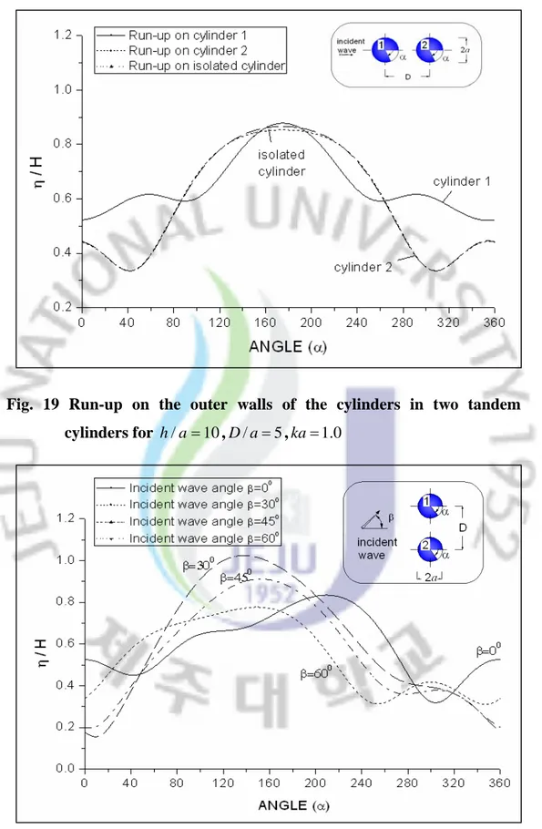
Fig. 19 Run-up on the outer walls of the cylinders in two tandem cylinders for , , ... 35

10 /a=

h D/a=5 ka=1.0

Fig. 20 Run-up on the outer wall of cylinder 1 in two transverse cylinders versus incident wave angle βfor h/a=10,D/a=5,ka=1.0... 35 Fig. 21 Run-up on the outer wall of cylinder 2 in two transverse cylinders versus

incident wave angle βfor h/a=10,D/a=5,ka=1.0... 36 Fig. 22 Run-up on the outer wall of cylinder 1 in two tandem cylinders versus incident

wave angle βfor h/a=10,D/a=5,ka=1.0... 36 Fig. 23 Run-up on the outer wall of cylinder 2 in two tandem cylinders versus incident

wave angle βfor h/a=10,D/a=5,ka=1.0... 37 Fig. 24 Free-surface elevation contour around two transverse cylinders for ,

, ... 39 10 /a= h 5 /a= D ka=1.0

Fig. 25 Wave height distribution around two transverse cylinders using three-dimensional graphic technique forh/a=10,D/a=5,ka=1.0... 39 Fig. 26 Free-surface elevation contour around two tandem cylinders for ,

, ... 40 10 /a= h 5 /a= D ka=1.0

Fig. 27 Wave height distribution around two tandem cylinders using three-dimensional graphic technique for h/a=10,D/a=5,ka=1.0 ... 40 Fig. 28 Geometries for: (a) Three cylinders in triangular array, (b) Three cylinders in

row array, (c) Three cylinders in column array

...

41 Fig. 29 Wave forces in x -direction acting on cylinder 1 and cylinder 2 in triangle array

versus wave number kafor h/a=10, D/a=5 ... ..42 Fig. 30 Wave forces in -direction acting on cylinder 1 and cylinder 3 in triangle

array versus wave number for y

ka h/a=10, D/a=5... ..43 Fig. 31 Wave forces in x -direction acting on cylinder 1 and cylinder 2 in row array

versus wave number kafor h/a=10, D/a=5 ... ..43 Fig. 32 Wave forces in -direction acting on the cylinders in row array versus wave

number for y

ka h/a=10, D/a=5... ..44 Fig. 33 Wave forces in x -direction acting on the cylinders in column array versus

wave number kafor h/a=10, D/a=5... ..44 Fig. 34 Wave forces in x -direction acting on cylinder 1 in triangular array versus the

ratio γ =2a /Dfor h/a=10... ..45 Fig. 35 Wave forces in x -direction acting on cylinder 2 in triangular array versus the

ratio γ =2a /Dfor h/a=10... ..46 Fig. 36 Wave forces in -direction acting on cylinder 1 in triangular array versus the

ratio y D a / 2 = γ for h/a=10... ..46 Fig. 37 Wave forces in x -direction acting on cylinder 1 in row array versus the ratio

D a / 2 =

γ for h/a=10... ..47 Fig. 38 Wave forces in x -direction acting on cylinder 2 in row array versus the ratio

D a / 2 =

γ for h/a=10... ..48 Fig. 39 Wave forces in y-direction acting on cylinder 1 in row array versus the ratio

D a / 2 =

γ for h/a=10... ..48 Fig. 40 Wave forces in x -direction acting on cylinder 1 in column array versus the

ratio γ =2a /Dfor h/a=10...49 Fig. 41 Wave forces in x -direction acting on cylinder 2 in column array versus the

Fig. 42 Wave forces in x -direction acting on cylinder 3 in column array versus the ratio γ =2a /Dfor h/a=10... ..50 Fig. 43 Wave forces in x -direction acting on cylinder 1 in triangular array with four

different incident wave angles β =00,300,450,600 for h/a=10,D/a=6 ..51 Fig. 44 Wave forces in x -direction acting on cylinder 2 in triangular array with four

different incident wave angles β =00,300,450,600 for h/a=10,D/a=6...52 Fig. 45 Wave forces in x -direction acting on cylinder 3 in triangular array with four

different incident wave angles β =00,300,450,600 for h/a=10,D/a=6...52 Fig. 46 Wave forces in x -direction acting on cylinder 1 in row array with four

different incident wave angles β =00,300,450,600 for h/a=10,D/a=6...53 Fig. 47 Wave forces in x -direction acting on cylinder 2 in row array with four

different incident wave angles β =00,300,450,600 for h/a=10,D/a=6...53 Fig. 48 Wave forces in x -direction acting on cylinder 3 in row array with four

different incident wave angles β =00,300,450,600 for h/a=10,D/a=6...54 Fig. 49 Wave forces in x -direction acting on cylinder 1 in column array with four

different incident wave angles β =00,300,450,600 for h/a=10,D/a=6...54 Fig. 50 Wave forces in x -direction acting on cylinder 2 in column array with four

different incident wave angles β =00,300,450,600 for h/a=10,D/a=6...55 Fig. 51 Wave forces in x -direction acting on cylinder 3 in column array with four

different incident wave angles β =00,300,450,600 for h/a=10,D/a=6...55 Fig. 52 Run-up on the outer walls of three cylinders in triangular array for

... ..57 , 10 /a= h 0 . 1 , 6 /a= ka= D

Fig. 53 Run-up on the outer walls of three cylinders in row array for

... ..58 , 10 /a= h 0 . 1 , 6 /a= ka= D

Fig. 54 Run-up on the outer walls of three cylinders in column array for

... ..59 , 10 /a= h 0 . 1 , 6 /a= ka= D

Fig. 55 Free-surface elevation contour around three cylinders in triangular array for ...61 0 . 1 , 6 / , 10 /a= D a= ka= h

Fig. 56 Wave height distribution around three cylinders in triangular array using three-dimensional graphic technique for h/a=10,D/a=6, ka=1.0... ..61 Fig. 57 Free-surface elevation contour around three cylinders in row array for

... ..62 0 . 1 , 6 / , 10 /a= D a= ka= h

Fig. 58 Wave height distribution around three cylinders in row array using three-dimensional graphic technique for h/a=10,D/a=6, ka=1.0... ..62 Fig. 59 Free-surface elevation contour around three cylinders in column array for

... ..63 0 . 1 , 6 / , 10 /a= D a= ka= h

Fig. 60 Wave height distribution around three cylinders in column array using three-dimensional graphic technique for h/a=10,D/a=6, ka=1.0... ..63

Summary

With the advances in the design and construction, various types of offshore structures are now commonly constructed with a composite configuration of several legs such as cylinders. Thus, the interaction between waves and multiple cylinders is becoming more and more important. The wave pressure and wave forces acting on the cylinders must be exactly estimate to evaluate the wave effects and the stability of structures.

The interaction between waves and offshore structures causes problems such as diffracted waves, reflected waves, and wave forces. Consider N large vertical circular cylinders placed on the bottom. As the incident waves impinge on each cylinder, the reflected waves move outward. On the sheltered side of the cylinders there will be a “shadow” zone where the wave fronts are bent around the cylinders, the so-called diffracted waves. The reflected waves and diffracted waves, combined, are usually called the scattered waves. The scattered waves of each cylinder can affect other cylinders in the group. This process is generally termed diffraction. By the process of diffraction the pressure around the cylinders will be changed and therefore the forces on the cylinders will be influenced. The problems could be dealt with the boundary value with the velocity potential.

There have been several studies dealing with the interaction of water waves and multiple cylinders. Twersky (1952) constructed a solution using an iterative procedure in which successive scattered waves by each of the cylinders were introduced at each other. This method was extended to the water wave case by Ohkusu (1974). The main drawback of the iterative procedure is that it rapidly becomes unmanageable as the number of the cylinders increases. Another approach is the direct matrix method, Spring and Monkmeyer (1974) proposed a solution for the interaction of water waves and the cylinders using eigenfunction expansion approach. They formulated the problem in terms of matrix equation and the solution is obtained by the inversion of the matrix.

Chakrabarti (1978) extended the work of Spring and Monkmeyer (1974), and obtained the solution for the diffracted wave of multiple cylinders by carrying out the analysis in a complex domain. Subsequently, Linton and Evan (1990) made a major simplification to the theory proposed by Spring and Monkmeyer (1974).

On the other hand, there are many studies to solve the diffraction problems of water waves by using boundary element method. Notably, Kim and Park (2007) studied a numerical analysis method to calculate the wave force on isolated vertical circular cylinder by boundary element method and the numerical results of their study are strong agreement with those of MacCamy and Fuchs (1954). Also, Kim and Cao (2008) studied wave forces acting on the two vertical cylinders and three vertical cylinders in water waves.

The boundary element method is divided into direct boundary element method and indirect boundary element method. The direct boundary element method derives from the integral equation by Green’s or Cauchy’s theory. This deriving process is solved by the special application of weighted residual method and it has general integral formulation. Derived integral equation is divided into two parts: the unknown functions and the derivatives of normal direction. One side of them generally has unknown values. The indirect boundary element method is derived integral equation in boundary conditions and is made operation function by singular value of governing equation. The coefficient that is involved operation function is unknown value in direct boundary element.

In this paper, a numerical analysis by boundary element method for calculating wave forces acting on multiple cylinders is presented. The numerical analysis method by Green function in direct boundary element method using velocity potential φ is developed. Attention has been concentrated on wave forces on N large vertical cylinders, having radius a and placed on the bottom. To verify this numerical method and to investigate the effect of the neighboring cylinders on the wave forces acting on a cylinder, two-cylinder configuration and three-cylinder configuration are used in this study. The wave forces acting on two vertical circular cylinders and three vertical

cylinders obtained from this numerical method are compared with those of Ohkusu (1974) and Chakrabarti (1978). The comparisons show that the computed results of this study are strong agreement with their results. Also in this study, several numerical examples are given to illustrate the effects of various parameters on the wave forces acting on the cylinders such as the cylinder spacing, the wave number, and the incident wave angle. The run-up and free surface elevation around two vertical cylinders and three vertical cylinders are also calculated.

Chapter 1

INTRODUCTION

1.1 Background

Recently with the advances in the design and construction, various types of offshore structures are now commonly constructed with a composite configuration of several legs such as cylinders. Thus, the interaction between waves and group of cylinders is becoming more and more important. The wave pressure and wave forces acting on the cylinders must be exactly estimate to evaluate the wave effects and the stability of structures.

The interaction between waves and offshore structures causes problems such as diffracted waves, reflected waves, and wave forces. Consider N large vertical cylinders placed on the bottom. As the incident waves impinge on each cylinder, the reflected waves move outward. On the sheltered side of the cylinders there will be a “shadow” zone where the wave fronts are bent around the cylinders, the so-called diffracted waves. The reflected waves and diffracted waves, combined, are usually called the scattered waves. The scattered waves of each cylinder in the group cylinders can affect other cylinders. This process is generally termed diffraction. By the process of diffraction the pressure around the cylinders will be change and therefore the forces on the cylinders will be influenced. The problems could be dealt with the boundary value with the velocity potential.

Linear diffracted wave theory which uses linear free surface conditions proposes many different methods because the linear diffracted wave theory is easy and simple. The diffracted wave problem of a vertical cylinder was initially developed by Havelock (1940) for the special case of infinite water depth. MacCamy and Fuchs (1954) proposed a linear theory for the problem of diffraction of plane waves from a vertical circular cylinder in the case of finite water depth and the results are exact to the first order.

After these researches, there have been many studies dealing with the interaction of waves and multiple cylinders. Twersky (1952) constructed a solution using an iterative procedure in which successive scattered waves by each of the cylinders were introduced at each other. This method was extended to the water wave case by Ohkusu (1974). The main drawback of the iterative procedure is that it rapidly becomes unmanageable as the number of the cylinders increases. Another approach is the direct matrix method, Spring and Monkmeyer(1974) proposed a solution for the interaction of water waves and the cylinders using eigenfunction expansion approach. They formulated the problem in terms of matrix equation and the solution is obtained by the inversion of the matrix. Chakrabarti (1978) extended the work of Spring and Monkmeyer, and obtained the solution for the diffracted wave of multiple cylinders by carrying out the analysis in a complex domain. Subsequently, Linton and Evan (1990) made a major simplification to the theory proposed by Spring and Monkmeyer.

1.2 Objectives

In recent years, the Boundary Element Method has emerged as a strong numerical method for investigating dynamic problems especially for radiation and scattering problems. The reasons are that the boundary integral equation satisfies radiation condition automatically and correctly, and for linear problems only the surface of the boundaries need to be discrestized.

The boundary element method is divided into direct boundary element method and indirect boundary element method. The direct boundary element method derives from the integral equation by Green’s or Cauchy’s theory. This deriving process is solved by the special application of weighted residual method and it has general integral formulation. Derived integral equation is divided into two parts: the unknown functions and the derivatives of normal direction. One side of them generally has unknown values. The indirect boundary element method is derived integral equation in boundary conditions and is made operation function by singular value of governing equation. The coefficient that is involved operation function is unknown value in direct boundary element.

Basing on boundary element method, there are many studies to solve the diffraction problems of water waves and structures. Notably, Kim and Park (2007) studied a numerical analysis method to calculate the wave forces on isolated vertical circular cylinder by boundary element method and their numerical results are strong agreement with those of MacCamy and Fuchs (1954). Also, Kim and Cao (2008) studied wave forces acting on two vertical cylinders and three vertical cylinders in water waves.

The main objectives of this study are to solve the diffraction problem of water waves by multiple cylinders by using boundary element method. In this study, a numerical analysis by boundary element method using velocity potential φ is developed. Once the wave velocity potential is known, the wave pressure, wave forces acting on the cylinders can be calculated by using it. Also, the wave run-up on the outer walls of the cylinders and free-surface elevation around the cylinders are calculated in this study.

1.3 Study Contents

A numerical analysis by boundary element method for calculating wave forces acting on multiple cylinders is described in this study. The numerical analysis method by Green function in direct boundary element method using velocity potential φ is developed. To verify this numerical analysis and to investigate the effect of the neighboring cylinders on the wave forces on a cylinder in the group, two-cylinder configuration and three-cylinder configuration are used in this study. The numerical results are carried out as follows:

(1) The wave forces acting on two cylinders and three cylinders are computed.

(2) To verify this method, the numerical results obtained from this study are compared with those of Ohkusu (1974) and those of Chakrabarti (1978).

(3) The effects of the cylinder spacing and wave angular frequency on the wave forces acting on the cylinders are analyzed.

(4) Also, the effects of incident wave angle on wave forces are investigated in this study.

(5) The run-up on outer walls of the cylinders and the free-surface elevation around the cylinders are also calculated.

Chapter 2

FORMULATION OF BOUNDARY ELEMENT ANALYSIS

2.1 Diffraction Phenomenon

This section will describe the diffraction phenomenon of waves by multiple vertical cylinders. Attention has been concentrated on the interaction of Nvertical cylinders with the incident waves where the cylinder diameter D is assumed to be much larger than the wave lengthL . As the incident waves impinge on each cylinder, the reflected waves move outward. On the sheltered side of the cylinders there will be a “shadow” zone where the wave fronts are bent around the cylinders, the so-called diffracted wave. The reflected waves and diffracted waves, combined, are usually called the scattered waves. The scattered waves of each cylinder can affect the other cylinders in the group. This process is generally termed diffraction. By the process of diffraction the pressure around the cylinders will be changed and therefore the forces on the cylinders will be influenced. It is generally accepted that the diffraction effect becomes important when the ratio D /L becomes larger than 0.2 (Issacson, 1979).

Normally, in the diffraction flow regime, the flow around the circular cylindrical bodies is unseparated. This can be shown by the following analysis:

The amplitude of the horizontal component of water-particle motion at the sea surface is as follows: ) tanh( 1 2 kh H a= × (1)

where H is the wave height, his the water depth andkis the wave number. L

k= 2π (2)

The Keulegan-Carpenter number for a vertical circular cylinder will then be:

) tanh( ) / ( ) / ( 2 kh L D L H D a KC= π = π (3)

The largest KCnumber is obtained when the maximum wave steepness is reached, namely whenH/L=(H/L)max. The latter may be given approximately as (Isaacson,

1979): ) tanh( 14 . 0 ) ( max kh L H ₌ (4) Therefore, the largest KCnumber that the body would experience may be written as: L D KC / 44 . 0 = (5)

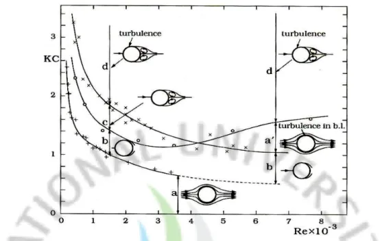
IfKCnumber is larger than this limiting value, the waves will break. Eq. (5) is plotted as a dashed line in Fig. 1. The vertical line D/L=0.2in Fig. 1 represents the boundary beyond which the diffraction effect becomes significant. Also, Fig. 1 indicates that the KCnumbers experienced in the diffraction flow regime are extremely small, namelyKC<2. Fig. 2 shows that forKC<2the flow will be unseparated in most of the case.

The preceding analysis suggests that the problems regarding the flow around and forces on a large body in the diffraction regime may be analyzed by potential theory in most of the situations, since the flow is unseparated.

Fig. 1 Different flow regimes in the (KC,D/L) plane. Adapted from Isaacson (1979)

Fig. 2 Regimes of flow around a smooth, circular cylinder in oscillatory flow

for smallKCnumbers (KC<3). Data: Circles from Sarpkaya (1986a);

crosses for Re<1000from Honji (1981) and crosses for Re>1000from Sarpkaya (1986a)

Fig. 3 Vortex-shedding regimes around a smooth circular cylinder in

oscillatory flow. Data: Lines, Sarpkaya (1986a) and Williamson (1985) and: squares from Justesen (1989)

2.2 Basic Equations and Boundary Conditions

Considering N vertical circular cylinders, having radiusa, are placed in the water of uniform depthh. The global Cartesian coordinate system(x,y,z)is defined with the origin located on the still-water level, the z axis directed vertically, xand y axis directed horizontally. The geometry of this problem is shown in Fig. 4.

As usual, it is assumed that the fluid is inviscid, incompressible, its motion is irritation. The cylinders subjected to a strain of regular wave of height H and angular frequency σ propagating at an angle βto the positive xaxis.

The velocity potentialΦ(x,y,z;t)can be defined by: ] ) , , ( [ ) ; , , ( i t e x y z e R t z y x = φ −σ Φ (6)

whereRe[]denotes the real part of a complex expression.

From the linear feature of potential flow, the total potentialφ can be written as the sum of incident wave velocity potential and scattered wave velocity potential:

s i φ

φ

φ = + (7)

where φ_iis the velocity potential of incident wave and φ_sis velocity potential of the scattered wave.

The incident wave velocity potentialφ_i is given as follows:

) sin cos ( cosh ) ( cosh 2 β β σ φ ik x y i e kh z h k H g i + + − = (8)

whereH/2is wave amplitude, g is the acceleration due to gravity, i is the imaginary unit i= −1, kis the wave number (k =2π/L; L : wave length). The quantityσ is the angular frequency and related to wave number k by the dispersion relation:

) tanh( 2 kh gk = σ (9)

It is known that the incident wave potential function in Eq. (8) satisfies boundary conditions.

Boundary problems by the formulation of scattered wave velocity potential φ_sare given as follows:

• Laplace equation: 0

2 =

∇ φs (in Ω ) (10.a)

• Free surface boundary condition:

0 2 = − ∂ ∂ s s g z φ σ φ (on ΓF) (10.b)

• Cylinder surface boundary condition:

n n i s ∂ ∂ − = ∂ ∂φ φ (on ΓH_m,m=1,...,N) (10.c) • Sea bed boundary condition:

0 = ∂ ∂ z s φ (on ΓB) (10.d)

• Radiation boundary condition:

0 } { lim − = ∂ ∂ ∞ → s s R R _R ikφ φ (on Γ_R) (10.e)

where Ω is the fluid region, ΓF is the free surface, ΓH_m,m=1,...,Nis the body surfaces

of N cylinders, ΓB is the sea bed, ΓR is the virtual boundary at infinity, n is the

outward unit normal on the boundary, and R= x2 +y2 .

The incident wave velocity potential can be defined as follows:

) sin cos ( , cosh ) ( cosh 2 β β σ φ ik x y i i i e kh z h k H g i + Ψ Ψ = + − = (11)

The scattered velocity potential is defined as follows: ) , ( cosh ) ( cosh 2 kh x y z h k H g i _s s Ψ + − = σ φ (12)

If the definitions of equations (11), (12) are substituted into Eqs.(10.a)∼(10.e), the boundary value problems with Ψ are obtained as follows: s

0 2 2Ψ + Ψ = ∇ s k s (in Ω ) (13.a) n n i s ∂ Ψ ∂ − = ∂ Ψ ∂ (on NS m m H , =1,..., ) (13.b) 0 } { lim − Ψ = ∂ Ψ ∂ ∞ → s s R R _R ik (on S∞) (13.c)

In Eqs. (13.a)∼(13.c), boundary value problems are two-dimension problems of y

x− plane as shown in Fig. 5. Finally, because of analyzing boundary value problems byΨ , the scattered wave velocity potential is calculated. Then the total velocity _s potential, wave pressure, and wave forces are calculated by using it.

a)

b)

Fig. 4 Definition of: a) Two vertical circular cylinders,

a) Two vertical circular cylinders

b) Three vertical circular cylinders

Fig. 5 Numerical model configurations:

2.3 Green Function

Green function plays an important role in the solution of partial differential equations, and is the key component to the development of boundary element method. Green function is a two-point function and it has peculiarity of 1/r, excludes special point in case r=0. Green function satisfies the Laplace equation and other boundary conditions except the boundary condition at the body surfaces.

) ( ) ( ) ( 2 ₌₋δ ₋ξ δ ₋η δ ₋ζ ∇ G x y z (in Ω ) (14) 0 2 = − ∂ ∂ G g z G σ (on ΓF) (15) 0 = ∂ ∂ z G (on ΓB) (16) 0 } { lim − ₀ = ∂ ∂ ∞ → _r ik G G r r (on ΓR) (17)

whereGis Green function,δ is Dirac Delta function and (ξ,η,ζ) is the coordinate of the point in the fluid region.

According to John (1950), the Green function is derived as follows: ) ( ) ( cosh } ) ( { 2 ) ( cosh ) ( ) , ( _{2 2 0 0}(1) ₀ 0 0 2 2 0 r k H z h hk k h h k k i Q P G + + − + − = ν ν ζ ν cosh ( ) ( ) } ) ( { ) ( cos ) ( 0 1 2 2 2 r k K z h k k k h k k n n n n n n n + − + + + +

∑

∞ = π ν ν ζ ν (18) 2 2 ) ( ) ( −ξ + −η = x y r

where, H_m(1): denotes the Hankel function of the first kind order m; K : denotes the _m modified Bessel function of the second kind order m; ....)k_n(n=0,1 : are the roots of the dispersion relation for free surface (k_ntan(k_nh)=−σ2/g)and are increasing size

...)

(k₁ < k₂ < . Also, ν =σ2/g ; P(ξ,η,ζ)andQ(x,y,z) are two points in the fluid region.

2.4 Derivation of Integral Equations

The basic step in boundary element method is transforming the governing differential equation into an integral equation. The governing Laplace’s equation for scattered wave potential φs(Eq. (10.a)) can be transformed into an integral equation by

using the method of weighted residual:

∫ ∫ ∫

∇ Ω= Ω 0 2 Gd s φ (19)

where the test functionGis Green function.

The integral equation of scattered wave potential in the domain Ω (Eq. 19) can be transformed into boundary integral equation on the boundary S via Green’s second identity and the result as follows:

∫ ∫

∫

∫ ∫

− ∂_∂ ∂ ∂ = Ω ∇ − ∇ Ω _n G _n ds G d G G s s S s s ) ( ) (φ 2 2φ φ φ (20)

where Sis the boundary of the fluid domain Ω ,n is the outward unit normal on the boundary. As shown in Fig. 4, the boundaries of the fluid domain are the cylinder surface boundariesΓ_Hm,m=1,...,N , free-surface boundaryΓ_F, sea bed boundaryΓ_B, and the virtual boundaryΓ_R. Thus Eq. (20) can be written as follows:

= Ω ∇ − ∇

∫ ∫ ∫

Ω ( s G G s)d 2 2 φ φ

_{∫ ∫}

_{∫ ∫}

∂ ∂ − ∂ ∂ + ∂ ∂ − ∂ ∂ ∑Γ Γ = ds z G z G ds n G n G _s s F s s m H ) ( ) ( N 1 m φ φ φ φ

∫ ∫

∫ ∫

Γ →∞ Γ ∂ ∂ − ∂ ∂ + ∂ ∂ − ∂ ∂ + R s s R s s B ds R G R G ds z G z G ) ( lim ) (φ φ φ φ (21)

Due to scattered wave potentialφs and Green function G satisfy the boundary

conditions at Γ_F, Γ_Band Γ_R, the integral equations at the boundaries Γ_F, Γ_Band Γ_Ron the right hand side of Eq. (21) are vanish. Therefore, Eq. (21) can be rewritten as follows:

∫ ∫ ∫

∇ − ∇ Ω= Ω ( s G G s)d 2 2 φ φ

_{∫ ∫}

∂ ∂ − ∂ ∂ ∑ = Γ _n G _n ds G _s s m H ) ( N 1 m φ φ (22)

∫ ∫ ∫

∇ Ω=− Ω ( ) 2 P Gd s s γ φ φ (23)

Finally substituting Eq. (19) and Eq. (23) into Eq. (22), the integral equation is obtained as follows:

∫ ∫

− ∂_∂ ∂ ∂ ∑ − = = Γ _n G _n ds G P s s m H s( ) N ( ) 1 m φ φ γφ (24)

where, γ =1 as the point P places in the domain Ω , and γ =1/2 as the point P places on the boundary of the domain.

In two-dimensional problems (Fig. 5), if the observation point i is presented over the boundary Splane, the boundary value problems of Eqs. (13.a)∼(13.c) with usingΨ , i Ψ s

are defined by the integral equation as shown in Eq. (25):

∫

∑ + _∞ ∂ Ψ ∂ − ∂ ∂ Ψ − = Ψ = S m H S s s si ds n G n G N 1 m ) ( 2 1 (25)

and rearranging, the results is derived as follows:

∫

∫

+_∞ ∑ + _∞ ∂ Ψ ∂ = ∑ ∂ ∂ Ψ + Ψ = = S m H S s S m H S s si ds n G ds n G N 1 m N 1 m 2 1 (26)

If observation point i is nearS_Hm , the Eq. (26) is the integral equation for S_∞. When S_∞ is near

m H

S with r>>1, kr ≅r , r ≅ , the Hankel function is given as R follows: ⎭ ⎬ ⎫ ⎩ ⎨ ⎧ ₋ ≅ ( 4) ) 1 ( 0 2 ) ( π π kR i e kR kr H ⎭⎬ ⎫ ⎩ ⎨ ⎧ ₋ ≅ ∂ ∂ ) 4 ( ) 1 ( 0 2 π π kR i e kR ik R H ( on S_∞) (27)

The integral term for S_∞ of Eq. (26) is substituted as follows:

∫

∞

∫

_∞ ∂ Ψ ∂ − ∂ ∂ Ψ S S s s Gds R ds R G

∫

∞ ⎟⎠ ⎞ ⎜ ⎝ ⎛ _{− Ψ} ∂ Ψ ∂ − = − S s s ikR i ds ik R R e e k i 4 2 4 1 π π

∫

⎟ ⎠ ⎞ ⎜ ⎝ ⎛ _{− Ψ} ∂ Ψ ∂ − = −π π π 2 0 4 2 4 1 ds ik R R e e k i s s ikR i (28) By substituting Eq. (28) into Eq. (13.c), the result is obtained as follows:

0 = ∂ Ψ ∂ − ∂ ∂ Ψ

∫

S_∞

∫

S_∞ s s Gds R ds R G (29) Therefore, the finally boundary integral equation on scattered wave potential is given as follows:

∫

∫

∑ ∂ Ψ ∂ = ∑ ∂ ∂ Ψ + Ψ = = N N m H S s m H S s si ds n G ds n G 1 m 1 m 2 1 (30)

Eq. (30) is the integral equation for the near curve S m N

m

H , =1,..., of the cylinder

surfaces and the scattered wave velocity potential on the boundary is derived by solving this equation.

The scattered wave potential in the domain Ω can be calculated after the scattered wave potential on the boundary has been known. If the observation point i is placed in the domainΩ , the integral equation for scattered wave potential is given as follows:

∫

∫

∑ ∂ ∂ Ψ − ∑ ∂ Ψ ∂ = Ψ = = N m N m Hm S e s m H S e s si ds n G Gds n 1 1 (31) where Ψ , _se n e s ∂ Ψ ∂

are the scattered wave potential and normal derivative of the scattered wave potential on the boundary.

Once the incident wave potential and scattered wave potential are known then the pressure, the wave forces and run-up on the cylinders can be calculated.

2.5 Formulation of Wave Force

The wave pressure acting on the cylinder is defined as follows: ] ) , , ( [ ) ; , , (x y z t R_e p x y z e i t P = −σ (32)

The Bernoulli equation is used to get the wave pressure: ) , , ( ) , , (x y z i x y z p = σρφ (33)

where ρis the water density.

The wave pressure is presented by using Ψ , _i Ψ as follows: _s ) ( cosh ) ( cosh 2 kh i s h z k H g p=ρ + Ψ +Ψ (34)

] [ _jm i t e m j R f e F = −σ (35)

The wave force in j direction is presented by using Ψ , i Ψ as follows: s

∫

∫

+ Ψ +Ψ = −h S_Hm i s j m j dz n ds kh h z k H g f 0 ( ) cosh ) ( cosh 2 ρ (36)

Finally, by integrating the wave force in z direction, the total wave force on the cylinder is defined as follows:

∫

Ψ +Ψ = m H S i s j m j n ds k kh H g f tanh ( ) 2 ρ (37)

Also the moment Mm_j in j direction on the cylinder mthis defined as follows:

∫

Ψ +Ψ × ⎭ ⎬ ⎫ ⎩ ⎨ ⎧ + − = m H S i s j m j n ds kh kh kh kh kh h H g M 2 ₂ ( ) ) cosh( ) ( ) cosh( 1 ) sinh( 2 ρ (38)

where n is the normal vector in the j direction element. _j

2.6 Formulation of Wave Run-up

The free-surface elevation is given by:

] ) , ( [ ) ; , (x y t Re x y e i t σ η η ₌ − on z=0 (39)

where η(x,y)is presented by using Ψ , i Ψ as follows: s

) ( 2 ) , ( i s H y x = Ψ +Ψ η (40)

Chapter 3

DISCRETIZATION OF INTEGRAL EQUATION

3.1 Discretization of the Boundary

To approximate the geometry, the surfaces of the cylinders are divided into N

boundary elementsΔ_i(i=1,2..N) . Inside each element Δ , the potential _i φ_s and the

normal derivative of velocity potential n

s

∂ ∂φ

are interpolated using the shape function and the node values. Therefore, the integral equation (24) leads to:

∫ ∫

∑

∫ ∫

∑

Δ = Δ = ∂ ∂ = ∂ ∂ + G P Q ds n P ds n Q P G P P i j N j j s i j N j j s i s ( , ) ) ( ) , ( ) ( ) ( 2 1 1 1 φ φ φ (41)

where P ,i Pj are the coordinate of the points located in the middle of element ithand

th

j respectively.

In two dimensional boundary value problems (Fig. 5), the surfaces of the cylinders

m H

S are divided into N boundary elementsΔ_i(i=1,2..N). The integral equation Eq. (30) leads to:

∫

∑

∫

∑

Δ = Δ = ∂ Ψ ∂ = ∂ ∂ Ψ + Ψ j i N j j s j i N j j s i s G P Q ds n P ds n Q P G P P 1 1 ) , ( ) ( ) , ( ) ( ) ( 2 1 (42)

3.2 The Collocation Method

The collocation method allows calculate the unknown boundary data from Eq. (42). The principle of collocation means to locate the load point sequentially at nodes of all the elements of the boundary such that the variable at the observation point coincides with the nodal value.

By collocating the observation point i with the nodes 1 to Nof the elements of the boundary, we can write Eq. (42) in matrix notation as follows:

⎟ ⎟ ⎟ ⎟ ⎟ ⎠ ⎞ ⎜ ⎜ ⎜ ⎜ ⎜ ⎝ ⎛ Ψ Ψ Ψ ⎟⎟ ⎟ ⎟ ⎟ ⎠ ⎞ ⎜⎜ ⎜ ⎜ ⎜ ⎝ ⎛ = ⎟⎟ ⎟ ⎟ ⎟ ⎠ ⎞ ⎜⎜ ⎜ ⎜ ⎜ ⎝ ⎛ Ψ Ψ Ψ ⎟ ⎟ ⎟ ⎟ ⎟ ⎠ ⎞ ⎜ ⎜ ⎜ ⎜ ⎜ ⎝ ⎛ ) ( ˆ ) ( ˆ ) ( ˆ . ... ... ) ( ) ( ) ( . ˆ ˆ ˆ ˆ ... ˆ ˆ ˆ ... ˆ ˆ 2 1 2 1 2 22 21 1 12 11 2 1 2 1 2 22 21 1 12 11 N s s s NN N N N N N s s s NN N N N N P P P G G G G G G G G G P P P G G G G G G G G G M L M O M M M L M O M M

(43)

In Eq. (43) the matrix element Gˆ and _ij G is defined as follows: _ij

⎪ ⎪ ⎩ ⎪⎪ ⎨ ⎧ ≠ ∂ ∂ = ∂ ∂ + =

∫

∫

Δ Δ j i j i ij j i ds n Q P G j i ds n Q P G G ) ( ) , ( ) ( ) , ( 2 1 ˆ ₍₄₄₎ and

∫

Δ = j i ij G P Q ds G ( , ) (45)

Also in Eq. (43), on the left hand sideΨs(Pi)is the velocity potential value of scattered wave at the node P of element i , and on the right hand side _i Ψˆ_s(P_i)is normal derivative value of velocity potential of scattered wave at the node P of element i . _i

3.3 Calculation of Matrix Element

On the left-hand side of Eq. (43), Gˆ is the derivative of Green function respect to _ij the normal drawn outwardly vector

→

n on the boundary and is defined as∂ /G ∂n . Also, on the right-hand side, Ψˆ_sis the derivative of velocity potential of scattered wave respect to the normal drawn outwardly vector

→

n on the boundary and is defined as n

s ∂

Ψ

∂ / . If the unit normal vector component nx,ny,nz is used, ∂ /G ∂n and

n

s ∂

Ψ

∂ / are defined as follows:

z G n y G n x G n n G z y x ∂ ∂ + ∂ ∂ + ∂ ∂ = ∂ ∂ (46) z n y n x n n s z s y s x s ∂ Ψ ∂ + ∂ Ψ ∂ + ∂ Ψ ∂ = ∂ Ψ ∂ (47)

In two dimensional x− plane,y ∂ /G ∂n and ∂Ψs /∂nare defined as follows: y G n x G n n G y x ∂ ∂ + ∂ ∂ = ∂ ∂ (48)

y n x n n s y s x s ∂ Ψ ∂ + ∂ Ψ ∂ = ∂ Ψ ∂ (49) where ∂ /G ∂x,∂ /G ∂y,∂ /G ∂z are the derivative of Green function respect to x,yandz.

x

s ∂

Ψ

∂ / ,∂Ψs /∂y, ∂Ψs/∂zare the derivative of scattered velocity potential respect to

z and ,y

x respectively.

To calculate coefficients Gˆ and ij G in Eq. (44) and Eq. (45), the integral equations ij

can be approximated as follows:

∫

Δ_jG(Pi,Q)ds ≅G(Pi,Pj)Δj (50) j j i j i n P P G ds n Q P G Δ ∂ ∂ ≅ ∂ ∂

∫

Δ ) , ( ) , ( (51) where Δ is the area of the element j . _j

3.4 Derivation of Green Function

Green function is the function which satisfies the boundary conditions Eqs.(14)∼(17). The eigenfunction expansion satisfies the free surface boundary condition Eq. (15) and sea bed boundary condition Eq. (16) is defined as follows:

⎪ ⎪ ⎩ ⎪ ⎪ ⎨ ⎧ = + + − = + + − = ,...) 2 , 1 (for cosh ) ( cosh ) ) ( 2 ) 0 (for cosh ) ( cosh ) ) ( 2 ) ( 2 2 2 0 0 2 2 0 2 0 n z k z h k k h k n z k z h k k h k z n n n n n ν ν ν ν φ (52)

The Delta function can be expanded as follows: ) ( ˆ ) ( ) ( 0 ζ φ φ ζ δ

∑

∞ = = − n n n z z (53)

where φˆ_n is the conjugate function of φ_n.

The Green function G is supposed as follows:

∑

∞ = = 0 ) ( ˆ ) ( ) , , , ( ) , ( n n n n x y z G Q P G ξ η φ φ ζ (54)

By substituting Eq. (54) into left hand side of basic equation (14) and substituting Eq. (53) into the right hand side, the result is obtained as follows:

∑

∑

∞ = ∞ = − − − = ± ∇ 0 0 2 2 ) ( ˆ ) ( ) ( ) ( ) ( ˆ ) ( ) ( n n n n n n n n n k G z x y z G φ φ ζ δ ξ δ η φ φ ζ (55)

where ∇ is the Laplace operator. In the parentheses, as 2 n=0the double sign is plus sign (+) and as n=1,2... the double sign is minus sign (-).

Therefore, the Green function, Gn(n=0,1,2...), need to satisfy condition as follows: ) ( ) ( 2 2 ± =−δ −ξ δ −η ∇ Gn knGn x y (56)

Eq. (56) is the two dimensional Helmholtz equation as n=0, and is the modified the two dimensional Helmholtz equation as n=1,2...

The fundamental solution for Helmholtz equation is obtained as follows:

) ... 2 , 1 , 0 ( ) ( 2 1 ) 0 ( ) ( 4 ) , ; , ( 0 0 ) 1 ( 0 ⎪ ⎪ ⎩ ⎪⎪ ⎨ ⎧ = = = n R k K n R k H i y x G n π η ξ (57) 2 2 ) ( ) ( −ξ + −η = x y R

where, H₀(1) denote the Hankel function of the first kind and order zero, K denote the ₀ modified Bessel function of the second kind and order zero.

Substituting Eq. (57) into Eq. (54) and using the eigenfunction,φn(n=0,1,2...), the three- dimensional Green function of wave motion can be derived as follows:

) ( ) cosh( } ) ( { 2 )) ( cosh( )) ( cosh( ) , ( 0 ) 1 ( 0 0 2 2 2 0 0 0 2 0 R k H h k h k h z h k h k k i Q P G ν ν ζ + − + + = ( ) ) ( cosh } ) ( { ) ( cos )) ( cos( 0 1 2 2 2 0 2 R k K h k k h z h k h k k n n n n n n

∑

∞ = + − + + + ν ν π ζ (58)

In which,cosh2(k₀h)−1 =1−tanh2(k₀h)and (cosh2k_nh)−1 =1+tanh2(k_nh) and the dispersion relation k₀tanhk₀h=ν and k_n tanhk_nh=−ν . By substituting these coefficients into Eq. (58), the result is derived as follows:

cosh ( ) ( ) } ) ( { 2 ) ( cosh ) ( ) , ( _{2 2 0 0}(1) ₀ 0 0 2 2 0 R k H z h hk k h h k k i Q P G + + − + − = ν ν ζ ν cosh ( ) ( ) } ) ( { ) ( cos ) ( 0 1 2 2 2 R k K z h k k k h k k n n n n n n n + − + + + +

∑

∞ = π ν ν ζ ν (59)

Chapter 4

NUMERICAL EXAMPLES

4.1 Wave Forces on Two Vertical Circular Cylinders

Fig. 6 demonstrates the geometries of two transverse cylinders and two tandem cylinders used in this study. The figure shows two cylinders, having radius a1=a2 =a,

subjected to incident wave comes from the left side. D is the distance between the centers of the cylinders. The wave exciting force on the cylinders, run-up and free-surface elevation around the cylinders 10adistance are calculated. In order to compare with the results of Chakrabarti (1978) and Ohkusu (1974), in all figures the wave forces are nondimensionalized by ρg(H /2)a2and the magnitude of run-up and free-surface elevation are nondimensionalized by wave height H .

a) b)

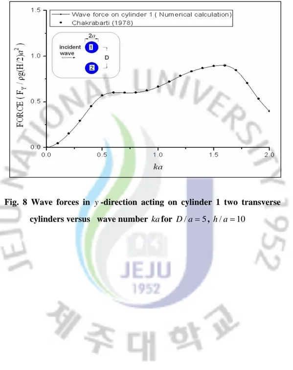
Fig. 7 and Fig. 8 show the wave forces in x-direction and y -direction acting on cylinder 1 in two transverse cylinders versus the wave number ka. Due to the symmetry of the geometry, the wave forces acting on cylinder 2 are the same. The wave forces acting on an isolate cylinder are also plotted for purpose of comparison. Fig. 7 shows that the wave forces on each cylinder in two transverse cylinders are higher than that on isolate cylinder because of the interaction of two cylinders. The numerical computation results of this study are strong agreement with those of Chakrabarti (1978).

Fig. 7 Wave forces in x-direction acting on cylinder 1 in two transverse

Fig. 8 Wave forces in y -direction acting on cylinder 1 two transverse

Fig. 9 shows the wave forces in x-direction acting on the cylinders in two tandem cylinders versus the wave number ka. The wave forces in y -direction on the cylinders in two tandem cylinders are zero. The results in Fig. 9 show that the wave forces on two cylinders reach maximum values near ka=0.5and the variation of the wave force on the front cylinder is more than that on the back cylinder. In two tandem cylinders, the wave forces on the rear cylinder are reduced by the shielding effect. Also, Fig. 9 shows that the numerical computation results of this study are strong agreement with those of Ohkusu (1974).

Fig. 9 Wave forces in x-direction acting on two tandem cylinders versus

4.1.1 The Effects of Cylinder Spacing on Wave Forces on Two Vertical

Circular Cylinders

The effects of the separation distance among two cylinders on the wave forces on two cylinders are also investigated in this study. Fig. 10 and Fig. 11 show the wave forces in x - direction and y - direction acting on each cylinder in two transverse cylinders versus the ratio γ =2a /D for three special wave numbers

0 . 1 and , 5 . 0 , 1 . 0 =

ka . In which, ais the radius of the cylinders, and D is the distance between the centers of the cylinders. In this geometry, γ =1 represents that the cylinders are touching each other, whereas γ =0 represents that the distance between two cylinder centers D→∞. Due to the symmetry of the geometry, the wave forces in

x- direction and y - direction acting on each cylinder 1 and cylinder 2 are the same. Fig. 12 shows the wave forces in x- direction acting on the cylinders in two tandem cylinders versus the ratio γ =2a /D for three special wave numbers

0 . 1 and , 5 . 0 , 1 . 0 =

ka . The wave force in y - direction is zero due to the symmetry of the geometry. In all figures, the corresponding wave forces acting on isolated cylinder are also plotted for the purpose of comparison.

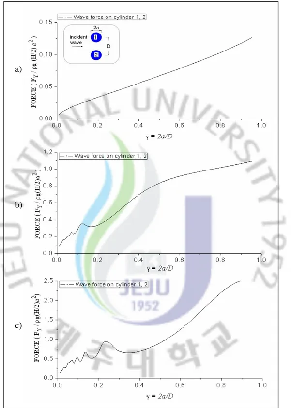
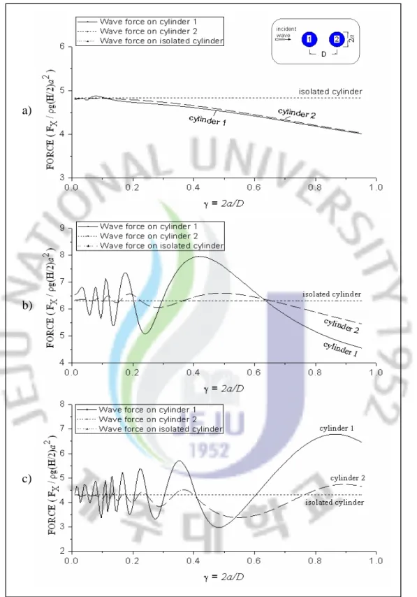
From the results shown in Fig. 10 to Fig. 12, as the cylinder spacing increases, the wave forces on the cylinders do not decrease linear to the wave forces on an isolated cylinder, however it oscillates around the wave forces on an isolated cylinder. The amplitude of oscillation is extremely large as the ratio γ ≥0.2. As the cylinder spacing approaches infinity, the wave forces on the cylinders reach the wave force amplitude on an isolated cylinder.

Fig. 12 shows that the wave forces on the rear cylinder are extremely less than the wave forces on the front cylinder because of the shielding effect.

a)

b)

c)

Fig. 10 Wave forces in x-direction acting on two transverse cylinders

versus ratio γ =2a /D for h/a=10: a) wave number ka=0.1; b) wave number ka=0.5; c) wave number ka=1.0

a)

b)

c)

Fig. 11 Wave forces iny -direction acting on two transverse cylinders

versus ratioγ =2a /D for h/a=10: a) wave number ka=0.1; b) wave number ka=0.5; c) wave number ka=1.0

a)

b)

c)

Fig. 12 Wave forces inx-direction acting on two tandem cylinders versus

ratioγ =2a /D for h/a=10: a) wave number ka=0.1; b) wave number ka=0.5; c) wave number ka=1.0

4.1.2 The Effects of Position of the Cylinders on Wave Forces on Two

Vertical Circular Cylinders

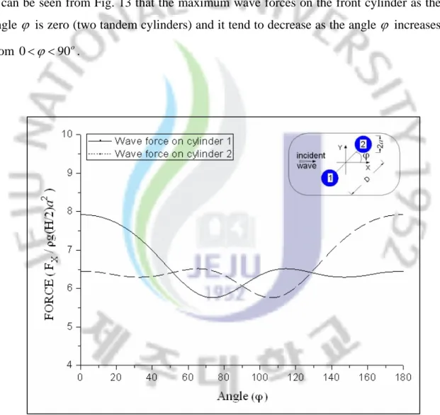
The effects of the position of the cylinders on the wave forces are also investigated in this study. Fig.13 shows the wave forces on the cylinders versus the variation of angle ϕ for special wave numberk =0.5, D/a=5, h/a=10. In which, ϕ is the counter-clockwise angle among the line joining the two cylinder centers and the x-axis. It can be seen from Fig. 13 that the maximum wave forces on the front cylinder as the angle ϕ is zero (two tandem cylinders) and it tend to decrease as the angle ϕ increases from 0<ϕ<90o.

Fig. 13 Wave forces inx-direction acting on two cylinders versus ratioϕ

4.1.3 The Effects of Incident Wave Angle on Wave Forces on Two

Vertical Circular Cylinders

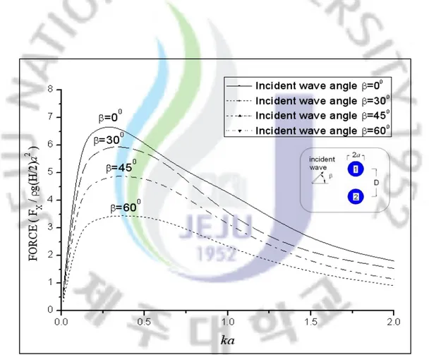
When incident wave is propagating at various anglesβ =00,300,450,600, the wave forces acting on the cylinders in two transverse cylinders and two tandem cylinders are computed as shown in Fig. 14 to Fig. 17. From the numerical computation results, the wave forces on the cylinders tend to decrease gradually as the incident wave angle increases in both two geometries. The variation of the wave forces on the cylinders in two tandem cylinders is larger than that on the cylinders in two transverse cylinders.

Fig. 14 Wave forces inx-direction acting on cylinder 1 in two transverse

cylinders with four different incident wave angles β =00,300,

0 0

60 ,

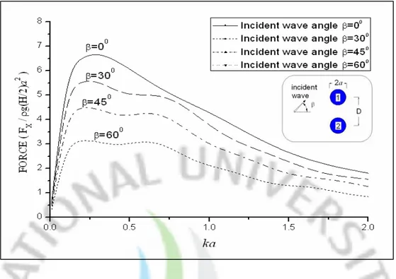
Fig. 15 Wave forces inx-direction acting on cylinder 2 in two transverse cylinders with four different incident wave angles β =00,300,

0 0

60 ,

45 forh/a=10,D/a=5

Fig. 16 Wave forces inx-direction acting on cylinder 1 in two tandem

cylinders with four different incident wave angles β =00,300,

0 0

60 ,

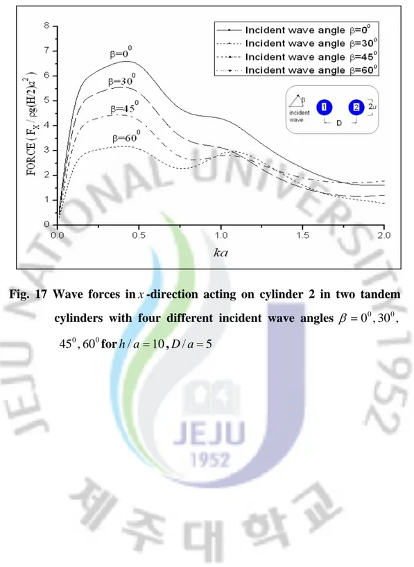
Fig. 17 Wave forces inx-direction acting on cylinder 2 in two tandem cylinders with four different incident wave angles β =00,300,

0 0

60 ,

4.1.4 Run-up on the Outer Walls of Two Vertical Circular Cylinders

The numerical computation results of run-up on the outer walls of the cylinders in two transverse and two tandem cylinders are shown in Fig. 18 and Fig. 19. The computation results show that due to the interaction of the cylinders, the run-up profiles of the cylinders are quite different from that of an isolated cylinder. In two tandem cylinders, the run-up on the front cylinder is higher than that on the back cylinder because the shielding effect. Also, the numerical computation results have strong agreement with those of Chakrabarti (1978).

Fig. 20 to Fig. 23 present the run-up on the outer walls of the cylinders in two transverse cylinders and two tandem cylinders for D/a=5, h/a=10, ka=1.0at four different incident wave angles β =0o,30o,45o,and60o.

Fig. 18 Run-up on the outer walls of the cylinders in two transverse cylinders for h/a =10,D/a=5,ka=1.0

Fig. 19 Run-up on the outer walls of the cylinders in two tandem cylinders for h/a =10,D/a=5,ka=1.0

Fig. 20 Run-up on the outer walls of cylinder 1 in two transverse cylinders versus incident wave angle βfor h/a=10,D/a=5,ka=1.0

Fig. 21 Run-up on the outer walls of cylinder 2 in two transverse cylinders versus incident wave angle βfor h/a=10,D/a=5,ka=1.0

Fig. 22 Run-up on the outer walls of cylinder 1 in two tandem cylinders versus incident wave angle βfor h/a=10,D/a=5,ka=1.0

Fig. 23 Run-up on the outer walls of cylinder 2 in two tandem cylinders versus incident wave angle βfor h/a=10,D/a=5,ka=1.0

4.1.5 Free-Surface Elevation around Two Vertical Circular Cylinders

The free-surface elevation contour around two transverse cylinders and two tandem cylinders for special wave number ka=1.0and incident wave angleβ =00is computed as shown in Fig. 24 and Fig. 26. The run-up on the cylinders in Fig. 18 and Fig. 19 is presented by the same value as in Fig. 24 and Fig. 26.

Fig. 25 and Fig. 27 show the wave height distribution around two transverse and two tandem cylinders using three-dimensional graphic technique.

incident wave

incide nt wave

Fig. 24 Free-surface elevation contour around two transverse cylinders for

h/a=10,D/a=5,ka=1.0

Fig. 25 Wave height distribution around two transverse cylinders using three-dimensional graphic technique for h/a=10,D/a=5,ka=1.0

incident wave

incide nt wave

Fig. 26 Free-surface elevation contour around two tandem cylinders for

10 /a =

h ,D/a=5,ka=1.0

Fig. 27 Wave height distribution around two tandem cylinders using three-dimensional graphic technique for h/a=10,D/a=5,ka=1.0

4.2 Wave Forces on Three Vertical Circular Cylinders

Fig. 28 demonstrates the geometries of three vertical circular cylinders used in this study. The figure shows three cylinders, having radiusa₁=a₂ =a₃ =a, subjected to the incident waves come from the left side. Three different geometries of three cylinders are used in this study: triangular array, row array and column array. The wave forces, run-up and free-surface elevation around three cylinders 10adistance are calculated.

a)

b) c)

Fig. 28 Geometries for: (a) Three cylinders in triangular array, (b) Three cylinders in row array, (c) Three cylinders in column array

Fig. 29 and Fig. 30 show the wave forces in x-direction and y -direction acting on cylinder 1 and cylinder 2 in triangular array versus wave number ka. Due to the symmetry of the geometry, the wave forces in x-direction and y -direction on the cylinder 1 and cylinder 3 are the same and the wave forces in y -direction on cylinder 2 is zero.

Fig. 31 and Fig. 32 show the wave forces in x-direction and y -direction acting on cylinder 1 and cylinder 2 in row array versus wave number ka. In this geometry, the wave forces in x-direction and y -direction on the cylinder 1 and cylinder 3 are the same and the wave forces in y -direction on cylinder 2 is zero.

Fig. 33 shows the wave forces in x-direction acting on the cylinders in column array versus wave numberka. The wave forces iny -direction are zero.

The computed results show that due to the interaction of the cylinders, the graphs of wave forces acting on the cylinders in three different geometries are quite different with the wave forces acting on isolated cylinder. In triangular array and column array, the wave forces reach the maximum value near ka=0.5. However in row array, the wave forces reach the maximum value near ka=0.3. Also, the computed results are strong agreement with those of Ohkusu (1974).

Fig. 29 Wave forces in x-direction acting on cylinder 1 and cylinder 2 in

Fig. 30 Wave forces in y -direction acting on cylinder 1 and cylinder 3 in

triangle array versus wave number kafor h/a=10, D/a=5

Fig. 31 Wave forces in x-direction acting on cylinder 1 and cylinder 2 in

Fig. 32 Wave forces in y -direction acting on the cylinders in row array

versus wave number kafor h/a=10, D/a=5

Fig. 33 Wave forces in x-direction acting on the cylinders in column

4.2.1 The Effects of Cylinder Spacing on Wave Forces on Three

Vertical Circular Cylinders

The effects of the cylinder spacing on the wave forces acting on three cylinders are also investigated in this study. Fig. 34 to Fig. 36 show the wave forces in x -direction and y --direction acting on the cylinders in triangular array versus the ratio

D a / 2 =

γ for three special wave numbers ka=0.1 ,0.5 ,1.0. In this geometry, the wave forces in x-direction and y -direction acting on cylinder 1 and cylinder 3 are the same, the wave forces in y -direction acting on cylinder 2 is zero.

The computed results show that the wave forces acting on three cylinders oscillate extremely large around the wave forces acting on an isolated cylinder as the ratioγ ≥0.2.

Also, the computed results are strong agreement with those of Chakrabarti (1978).

Fig. 34 Wave forces in x-direction acting on cylinder 1 in triangular

Fig. 35 Wave forces in x-direction acting on cylinder 2 in triangular array versus the ratio γ =2a /Dfor h/a=10

Fig. 36 Wave forces in y -direction acting on cylinder 1 in triangular

Fig. 37 to Fig. 39 show the wave forces in x-direction and y -direction acting on three cylinders in row array versus the ratio γ =2a /Dfor three special wave numbers

0 . 1 , 5 . 0 , 1 . 0 and

ka= . The wave forces in x -direction and y -direction acting on cylinder 1 and cylinder 3 are the same, the wave forces iny -direction acting on cylinder 2 is zero.

Fig. 37 Wave forces in x-direction acting on cylinder 1 in row array