저작자표시 2.0 대한민국 이용자는 아래의 조건을 따르는 경우에 한하여 자유롭게 l 이 저작물을 복제, 배포, 전송, 전시, 공연 및 방송할 수 있습니다. l 이차적 저작물을 작성할 수 있습니다. l 이 저작물을 영리 목적으로 이용할 수 있습니다. 다음과 같은 조건을 따라야 합니다: l 귀하는, 이 저작물의 재이용이나 배포의 경우, 이 저작물에 적용된 이용허락조건 을 명확하게 나타내어야 합니다. l 저작권자로부터 별도의 허가를 받으면 이러한 조건들은 적용되지 않습니다. 저작권법에 따른 이용자의 권리는 위의 내용에 의하여 영향을 받지 않습니다. 이것은 이용허락규약(Legal Code)을 이해하기 쉽게 요약한 것입니다. Disclaimer 저작자표시. 귀하는 원저작자를 표시하여야 합니다.
공학석사 학위논문
UDR 을 위한 하드웨어 설계 연구
A Study on a Hardware Design for an
Underwater Disk Robot
지도교수 최 형 식
2012 년 2 월
한국해양대학교 대학원
기 계 공 학 과
本 論文을 Tran Ngoc Huy 의 工學碩士 學位論文으로 認准함.
위원장 유 삼 상 (인)
위 원 최 형 식 (인)
위 원 김 준 영
(인)
2012 년 2 월
한국해양대학교 대학원
1
Acknowledgement
I would like to express my deep gratitude to my supervisor Professor Hyeung-Sik Choi, for his invaluable help, encouragement, and patience during the master course in Department of Mechanical Engineering. His insight, vision, suggestions, and special behavior of brisk style in work has impressed to me and helped me to archive success in research and study.
I am grateful to Professor Sam-sang You, major of Refrigeration, Air-conditioning and Energy System Engineering; Professor Joon-Young Kim, major of Marine Equipment Engineering; Professor Jae-hyun Jeong, major of Mechanical System Engineering... They all helped and taught me immeasurably in detailing comments for my study in Korea Maritime University, Korea.
Special thanks to all the members of Intelligent Robot & Automation Lab (KIAL) for giving me a helpful, active and comfortable environment which conducts my scientific pursuits.
I closely express my thanks to Korean and Vietnamese friends for their friendliness, sharing, and confidence.
Last but by no means least, it is warmly that I would like to thank my parents, my brother, and my sister for their constant support and encouragement.
Korea Maritime University, Pusan, Korea February 1st 2012
2
A Study on a Hardware Design for an
Underwater Disk Robot
Tran Ngoc Huy
Department of Mechanical Engineering Graduate School of Korea Maritime University, 2012
Abstract
This paper introduces the new development of an Underwater Disk Robot (UDR) performing robust underwater motion under multi-directional disturbances. This is a new idea to overcome the underwater robot disadvantages which are motions, disturbance effect on the side. The UDR is six-DOF model composed of a frame structure include control system, sensor system ,four vertical actuators for heaving, rolling, pitching, rotating motion and three low-cost thrusters were developed for robust surging, swaying motion. Three thrusters are disposed symmetrically by 120 degrees to navigate along any directions by robust vector propulsion control scheme. The UDR is designed as a disk shaped vehicle to be less affected by external disturbances such as currents and waves. A control system including PID motion controller and sensor systems using depth sensor and low-cost AHRS sensor are developed.
3
Table of Contents
List of Tables ... 4
Chapter 1 Introduction ... 7
1.1 Motivation ... 7
1.2 Aim and Scope ... 9
Chapter 2 Modeling of the UDR ... 10
2.1 Design UDR ... 10
2.2 Elements of the governing equations ... 13
2.3 Vector actuation analysis ... 18
Chapter 3 Hardware Design ... 20
3.1 Microcontroller ... 20
3.2 Actuators and Equipments ... 23
3.3 Sensor ... 31
3.4 UDR System ... 37
Chapter 4 Theoretical Background ... 39
4.1 Attitude and Heading representation ... 39
4.2 Kalman Filter ... 43
4.3 Proportional Integral Differential (PID) control ... 46
Chapter 5 Experiments and Results ... 50
5.1 Developed AHRS ... 50
5.2 UDR Experiments ... 54
Chapter 6 Conclusion ... 59
4
List of Tables
Table 2.1: Mechanism specification of the UDR... 12
Table 3.1: Specifications of DSP. ... 22
Table 3.2: Summarize H-bridge operation. ... 24
Table 3.3: Specifications of RX-64 ... 27
Table 3.4: Comparison with present products. ... 30
Table 3.5: Thrust test results. ... 30
Table 4.1: PID tuning. ... 47
Table 4.2: Effects of increasing a parameter independently. ... 48
5
List of Figures
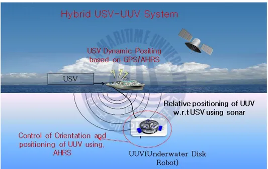
Fig. 1.1: Hybrid USV-UUV system. ... 8
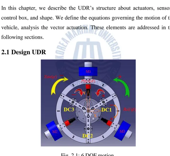
Fig. 2.1: 6 DOF motion. ... 10
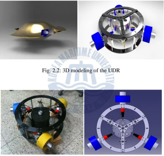
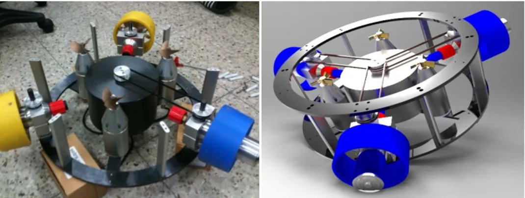
Fig. 2.2: 3D modeling of the UDR ... 11
Fig. 2.3: Thrusters are disposed symmetrically by 120 degrees ... 11
Fig. 2.4: The vertical actuators ... 12
Fig. 2.5: Control box ... 12
Fig. 2.6: UDR Body-fixed and Inertial Coordinate systems ... 14
Fig. 2.7: The unit vector. ... 18
Fig. 2.8: Vector actuation analysis. ... 19
Fig. 3.1: Roadmap of TMS320C2000 DSC’s. ... 20
Fig. 3.2: Broad C28x Application Base. ... 21
Fig. 3.3: The DSP nomenclature decoder. ... 22
Fig. 3.4: Maxon DC motor. ... 23
Fig. 3.5: H-bridge circuit. ... 23
Fig. 3.6: DC motor motion control system. ... 24
Fig. 3.7: Specifications of DC Motor Driver. ... 25
Fig. 3.8: Define Dynamixel RX-64. ... 26
Fig. 3.9: Dynamixel RC motor. ... 26
Fig. 3.10: BLDC driver. ... 29
Fig. 3.11: Specification of developed thrusting system. ... 29
Fig. 3.12: Configuration of experimental apparatus. ... 30
Fig. 3.14: Internal circuit diagram of pressure sensor. ... 31
Fig. 3.13: Model PSH. ... 31
Fig. 3.15: Attitude heading reference system. ... 32
Fig. 3.16: Attitude heading reference system block schematic. ... 33
Fig. 3.17: Prototype board in development process. ... 33
Fig. 3.18: Axial Orientation. ... 34
Fig. 3.19: Functional block diagram. ... 34
Fig. 3.20: TMS320F28335 pins, SPI port. ... 35
Fig. 3.21: CAN and Serial port. ... 35
Fig. 3.22: AHRS’s Interface. ... 36
Fig. 3.23: UDR system diagram. ... 37
6
Fig. 4.2: Euler angle sequence. ... 41
Fig. 4.3: The Discrete Kalman Filter Algorithm. ... 44
Fig. 4.4: The operation of the Kalman filter. ... 45
Fig. 4.5: A block diagram of a PID controller. ... 47
Fig. 5.1: Flow diagram of AHRS system. ... 50
Fig. 5.2: Roll angle without filter (Max Error= 6º). ... 51
Fig. 5.3: Roll angle after filter (Max Error= 0.5º). ... 51
Fig. 5.4: Pitch angle without filter (Max Error= 5º). ... 52
Fig. 5.5: Pitch angle after filter (error= 0.6º). ... 52
Fig. 5.6: Yaw angle without filter (Max Error= 12º). ... 53
Fig. 5.7: Yaw angle after filter (Max Error= 1.5º). ... 53
Fig. 5.8: UDR in water-tank. ... 54
Fig. 5.9: The Roll angle. ... 54
Fig. 5.10: The Pitch angle. ... 55
Fig. 5.11: PID for Title and Depth control... 55
Fig. 5.12: Control Depth and keep Roll=Pitch=10 degree. ... 56
Fig. 5.13: Control Title to Roll=Pitch=0 degree with disturbance. ... 56
Fig. 5.14: Control Roll=Pitch=0 degree, Depth=0.2m with disturbance ... 57
7
Chapter 1 Introduction
1.1 Motivation
Ocean is cradle of life, treasury resource and transportation artery. In the 21st century, we will face three challenges, such as the contradiction between population explosion and limited living space, between exhausted land resource and growing requirement of social production, between eco-environmental degradation and human development. Beside that, there exist sea regions with dangerous mines that should be eradicated for humanitarian reasons. It is clearly convenient and useful to use underwater robots such as USV, ROV, AUV [1] for oceanographic, bathymetric survey costal area, support works of the underwater vehicles by aiding the communication, localization and mine countermeasures, with no risks for humans.
Remotely operated underwater vehicles (ROVs) are unoccupied, highly maneuverable underwater robots operated by a person aboard a surface vessel. They are linked to the ship by a group of cables that carry electrical signals back and forth between the operator and the vehicle. Most are equipped with at least a video camera and lights. Additional equipment is commonly added to expand the vehicle’s capabilities. These may include a still camera, a manipulator or cutting arm, water samplers, and instruments that measure water clarity, light penetration, and temperature. The
8
disadvantages of using an ROV include the fact that the human presence is lost, making visual surveys and evaluations more difficult, and the lack of freedom from the surface due to the ROV’s cabled connection to the ship.
An autonomous underwater vehicle (AUV) is a robot which travels underwater without requiring input from an operator. It has two significant limiting factors. Firstly, batteries. Limitation in battery power restricted either endurance or the sensors that the vehicle could carry. Secondly, vehicle navigation and control.
Fig. 1.1: Hybrid USV-UUV system.
Generally, the underwater vehicle either tend to be cumbersome and complex to run, or operationally simple, but not quite suitable platforms for deep water imaging and weak to side disturbance effects [2] [3] [4]. Aware of the currently existing capabilities of underwater robot, we have initially designed and developed Underwater Disk Robot (UDR) which has manned or unmanned ability, enable the operator to record imagery below the ocean surface. With the disk shape, symmetric redundant actuators and vector
9
actuation system it can be the least side disturbance effect, robust underwater motion under multi-directional disturbances, swift motion to any directions such as horizontally, vertically and laterally.
1.2 Aim and Scope
In this study, it is desired to establish the modeling of UDR with symmetric structure and actuator’s locations. The hardware system is designed to operate UDR by using DSP microcontroller, developed low-cost AHRS sensor. Further, it is aimed to control heaving, rolling, pitching, rotating motion through PID controller and Kalman filter.
10
Chapter 2 Modeling of the UDR
In this chapter, we describe the UDR’s structure about actuators, sensors, control box, and shape. We define the equations governing the motion of the vehicle, analysis the vector actuation. These elements are addressed in the following sections.
2.1 Design UDR
Fig. 2.1: 6 DOF motion.
The UDR is designed as a disk shaped vehicle (Figure 2.1) to be less affected by external disturbances such as currents, wave. Especially, with three thrusters disposed symmetrically by 120 degrees (Figure 2.2) are used
11
to navigate along any directions by robust vector propulsion control scheme. They can control UDR for surging, swaying motion. And four vertical actuators which include three Z-cylinder DC Motors and RC Motor, perform for heaving, rolling, pitching, and rotating motion (Figure 2.3).
Fig. 2.2: 3D modeling of the UDR
12
Fig. 2.4: The vertical actuators
The control box is designed to contain the RC motor (support in rotating motion), depth sensor, IMU sensor , and DSP board which is programmed for controlling UDR and communicate with computer (Figure 2.4). The below table 2.1 will show mechanism specification of the UDR.
Fig. 2.5: Control box
Table 2.1: Mechanism specification of the UDR
Parameter Value Weight 22kg Diameter 0.475m Height 0.177m Depth 50m Speed 2 knots (1.028m/s) D.O.F 6
13
2.2 Elements of the governing equations
In this chapter, we define the equations governing the motion of the vehicle [5]. These equations consist of the following elements:
Kinematics: the geometric aspects of motion Rigid-body Dynamics: the vehicle inertia matrix Mechanics: forces and moments causing motion These elements are addressed in the following sections. 2.2.1 Vehicle Kinematics
The motion of the body-fixed frame of reference is described relative to an inertial or earth-fixed reference frame. The general motion of the vehicle in six degree of freedom can be described by the following vectors:
1 [ ] ; T x y z 2 [ ]T 1 [ ] ; T v u v w v2 [p q r]T 1 [ ] ; T X Y Z 2 [K M N]T (2.1) Where:
describes the position and orientation of the vehicle with respect to the inertial or earth-fixed reference frame.
v describes the translational and rotational velocities of the vehicle with respect to the body-fixed reference frame.
describes the total forces and moments acting on the vehicle with respect to the body-fixed reference frame.14
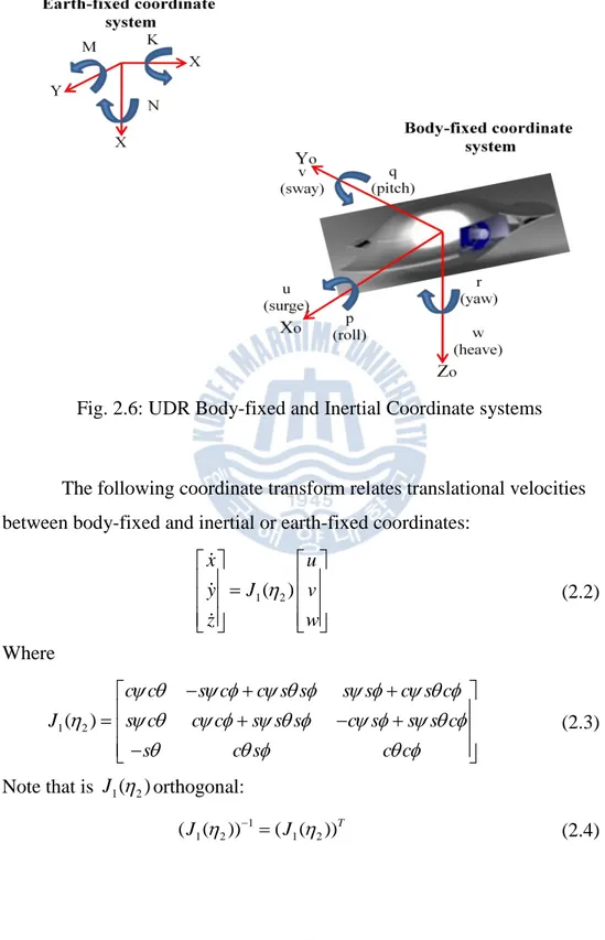
See Figure 2.6 for a diagram of the vehicle coordinate system.
Fig. 2.6: UDR Body-fixed and Inertial Coordinate systems
The following coordinate transform relates translational velocities between body-fixed and inertial or earth-fixed coordinates:
1( 2) x u y J v z w (2.2) Where 1( 2) c c s c c s s s s c s c J s c c c s s s c s s s c s c s c c (2.3)
Note that is J1(2)orthogonal:
1
1 2 1 2
15
The second coordinate transform relates rotational velocities between body-fixed and earth-fixed cooridinates:
2( 2) p J q r (2.5) Where 2 2 1 ( ) 0 0 / / s t c t J c s s c c c (2.6)
Note that J2(2) is not defined for pitch angle 0
90
. This is not a problem, as the vehicle motion does not ordinarily approach this singularity. If we were in a situation where it became necessary to model the vehicle motion through extreme pitch angles, we could resort to an alternate kinematic representation such as quaternions or Rodriguez parameters.
2.2.2 Vehicle Rigid-body Dynamics
The locations of the vehicle centers of gravity and buoyancy are defined in terms of the body-fixed coordinate system as follows:
g G g g x r y z b B b b x r y z (2.7)
In the following sections, we will show that the 6DOF nonlinear dynamic equations of motion can be conveniently express as:
( ) ( ) ( )
MC D g (2.8) Where
M: Inertia matrix (including added mass)
( )
16
( )
D : Damping matrix
( )
g : Vector of gravitational forces and moments
: Vector of control inputsThe parameterization of the rigid-bod inertia matrix M
11 12 21 22 3 3 0 ( ) ( ) 0 0 0 0 0 0 0 0 0 0 0 0 x G G G G G G G G G G x xy xz G G yz y yz G G zx zy z M M M M M mI mS r mS r I m mz my m mz mx m my mx mz my I I I mz mx I I I my mx I I I (2.9)
We can always parameterize the Coriolis and centripetal matrix by defining:
3 3 11 1 12 2 11 1 12 2 21 1 22 2 0 ( ) ( ) ( ) ( ) 0 0 0 ( ) ( ) ( ) 0 0 0 ( ) ( ) ( ) 0 0 0 ( ) ( ) ( ) ( ) ( ) ( ) 0 x G G G G G G G G G G G G G G G G yz xz z yz S M M C S M M S M M m y q z r m x q w m x r v m y p w m z r x p m y r u m z p v m z q u m x p y q m y q z r m y p w m z p v I q I p I r I r ( ) ( ) ( ) 0 ( ) ( ) ( ) 0 xy y G G G G yz xz z xz xy x G G G G yz xy y xz xy x I p I q m x q w m z r x p m z q u I q I p I r I r I q I p m x r v m y r u m x p y q I r I p I q I r I q I p (2.10)
Given that the origin of the body-fixed coordinate system is located at the center of buoyance.Form equation (2.8) we have the equations of motion for a rigid body in six degrees of freedom, defined in terms of body-fixed coordinates:
17 2 2 2 2 2 2 2 2 [ ( ) ( ) ( )] [ ( ) ( ) ( )] [ ( ) ( ) ( )] ( ) ( ) ( ) ( ) [ ( g g g ext g g g ext g g g ext xx zz yy xz yz xy g m u vr wq x q r y pq r z pr q X m v wp ur y r p z pr p x qp r Y m w uq vp z p q x rp q y rq p Z I p I I qr r pq I r q I pr q I m y w
2 2 2 2 ) ( )] ( ) ( ) ( ) ( ) [ ( ) ( )] ( ) ( ) ( ) ( ) [ ( ) ( )] g ext yy xx zz xy xz yz g g ext zz yy xx yz xy xz g g ext uq vp z v wp ur K I q I I rp p qr I p r I qp r I m z u vr wq x w uq vp M I r I I pq q rp I q p I rq p I m x v wp ur y u vr wq N
(2.11)Where m is the vehicle mass. The first three equations represent translational motion, the second three rotational motion. Note that these equations neglect the zero-valued center of buoyancy terms.
Given the body-fixed coordinate system centered at the vehicle center of buoyancy, we have the following, diagonal inertia tensor.
0 0 0 0 0 0 xx o yy zz I I I I (2.12)
This is based on the assumption, Ixy,I ,and xz Iyz are small compared
to the moments of inertia I ,xx Iyy, and I . zz
18 2 2 2 2 2 2 [ ( ) ( ) ( )] [ ( ) ( ) ( )] [ ( ) ( ) ( )] ( ) [ ( ) ( )] ( g g g ext g g g ext g g g ext xx zz yy g g ext yy m u vr wq x q r y pq r z pr q X m v wp ur y r p z pr p x qp r Y m w uq vp z p q x rp q y rq p Z I p I I qr m y w uq vp z v wp ur K I q
) [ ( ) ( )] ( ) [ ( ) ( )] xx zz g g ext zz yy xx g g ext I I rp m z u vr wq x w uq vp M I r I I pq m x v wp ur y u vr wq N
(2.13) 2.2.3 Vehicle MechanicsIn the vehicle equations of motion, external forces and moments are included:
ext hydrostatic lift drag control
F F F F F
(2.14)These forces are described in terms of vehicle coefficients. They are based on a combination of theoretical equations and empirically-derived formulae.
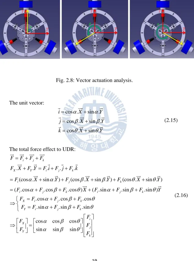
2.3 Vector actuation analysis
Fig. 2.7: The unit vector.
Three thrusters make the forces: F F Fi, j, k The total force:
F
F XX. F YY.19
Fig. 2.8: Vector actuation analysis.
The unit vector:
cos . sin . cos . sin . cos . sin . i X Y j X Y k X Y (2.15)
The total force effect to UDR:
. . . . . i j k X Y i j k F F F F F X F Y F i F j F k
(cos . sin . ) (cos . sin . ) (cos . sin . ) ( .cos .cos .cos ) ( .sin .sin .sin )
i j k i j k i j k F X Y F X Y F X Y F F F X F F F Y
.cos .cos .cos
.sin .sin .sin
cos cos cos
sin sin sin
X i j k Y i j k i X j Y k F F F F F F F F F F F F F (2.16)
20
Chapter 3 Hardware Design
In this chapter, we will explain about UDR system. There are DSP micro-controller, actuators (Thrusters, RC Motor, DC Motors), motor driver, and sensors (depth, AHRS). The AHRS is developed and applied to control system.
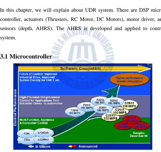
3.1 Microcontroller
Fig. 3.1: Roadmap of TMS320C2000 DSC’s.
Ti’s C2000 devices [6] are 32 bit microcontrollers with high performance integrated peripherals designed for real-time control applications. Its math-optimized core gives designers the means to improve
21
system efficiency, reliability, and flexibility. Powerful integrated peripherals make C2000 devices the perfect single-chip control solution. C2000’s development tools strategy and software create an open platform with the goal of maximizing usability and minimizing development time.
C2000 apllications:
Digital motor control Renewable energy systems Digital power conversion Adaptive lighting systems Automotive applications
Power line communications etc.
Fig. 3.2: Broad C28x Application Base.
In UDR, we used two kind of DSP: TMS320F28335 and TMS320F2812. The device nomenclature decoder is shown by following figure.
22
Fig. 3.3: The DSP nomenclature decoder.
Table 3.1: Specifications of DSP.
Parameter F28335 F2812
CPU 32 bit 32 bit
Floating-point Unit √ MIPS 150 150 RAM (words) 34K 18K ROM (words) Flash (words) 256K 128K BootROM (words) 8K 4K CAP/QEP 6/2 6/6 PWM 18 16 TIMER 3 7
ADC Resolution 12-bit 12-bit
Channels 16 16 Conv time 80ns 200ns McBSP √ √ EXMIF √ √ Watch Dog √ √ SPI √ √ SCI (UART) 3 2 CAN 2 2
Volts (V) 3.3 I/O 3.3 I/O
# I/O 88 56
Package 176 LQFP 179 BGA
176 LQFP 179 BGA
23
3.2 Actuators and Equipments
3.2.1 DC Motor
Fig. 3.4: Maxon DC motor. Specifications:
Nominal Voltage : 24V No load speed : 8810rpm No load current : 164mA Nominal torque : 1020mNm Terminal inductance : 0.119mH Power : 60W Weight of motor : 238g Motor driver
We designed DC Motor driver which was based on H-bridge circuit.
24 Table 3.2: Summarize H-bridge operation.
High side left High side right Lower left Lower right Description
On Off Off On Clockwise Off On On Off
Counter-clockwise On On Off Off Brake Off Off On On Brake
Motor motion controller is shown in Fig, and Ti’s TMS320F2812 processor controls the motor driver that consists of 500W total for two DC servo motor. In addition, with the built current sensor in motor driver we can apply PID control algorithm and the trapezoidal speed method.
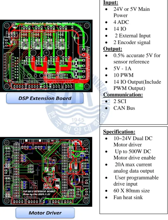
25 Specifications:
Fig. 3.7: Specifications of DC Motor Driver. Input: 24V or 5V Main Power 4 ADC 14 IO 2 External Input 2 Encoder signal Output: 0.5% accurate 5V for sensor reference 5V - 1A 10 PWM 14 IO Output(Include PWM Output) Communication: 2 SCI CAN Bus Specification: 10~24V Dual DC Motor driver Up to 500W DC
Motor drive enable 20A max current
analog data output User programmable
drive input 60 X 80mm size Fan heat sink
26 3.2.2 RC Motor (Dynamixel RX-64)
Dynamixel is a robot-only Smart Actuator with a new concept integrating speed reducer, controller, driver, network function, etc. into one module.
Fig. 3.8: Define Dynamixel RX-64.
Fig. 3.9: Dynamixel RC motor. Strong points of Dynamixel:
Torque: In spite of the compact size, it generates relatively big Torque by way of the efficient speed reduction
27
Close control: It can control location and speed with the resolution of 1024
Elasticity setting: It can set up the extent of elasticity when controlling position with compliance driving.
Position, speed: It can read the current position and speed
Communication: Dynamixel with a unique ID is controlled by packet communication on a BUS and supports networks such as TTL, RS485, and Can depending on the type of model.
Distribution control: Since the main processor can set speed, position, compliance, torque, etc. simultaneously with a single command packet.
Safety device: Is has the function, which notifies when internal temperature, torque, supplied voltage, etc. deviate from what the user has set, and the function, which allows it to cope with situation by itself.
Table 3.3: Specifications of RX-64
Parameter RX-64
Weight (g) 125 Dimension (mm) 40.2x61.1x41.0 Gear reduction ratio 1/200
Applied voltage (V) At 15V At 18V Final reduction stopping torque
(kgf.cm)
64.4 77.2
Speed (sec/60 degrees) 0.188 0.157
Resolution: 0.290
Running degree: 3000, Endless Turn Voltage: 12V-21V
28 Max Current: 1200mA Running Temp: 5 C0 _85 C0
Command signal: Digital Packet
Protocol: RS485 Asynchronous Serial Communication (8bit, 1stop, No parity)
Link: RS485 Multi Drop Bus ID: 254 ID (0_253)
Communication Speed: 7343 bps_1 Mbps
Sensing & measuring: Position, Temperature, Load, Input Voltage, etc. Material Quality: Full metal gear, engineering plastic body
Motor: Maxon RE-MAX Standby current: 50mA
3.2.3 Thruster
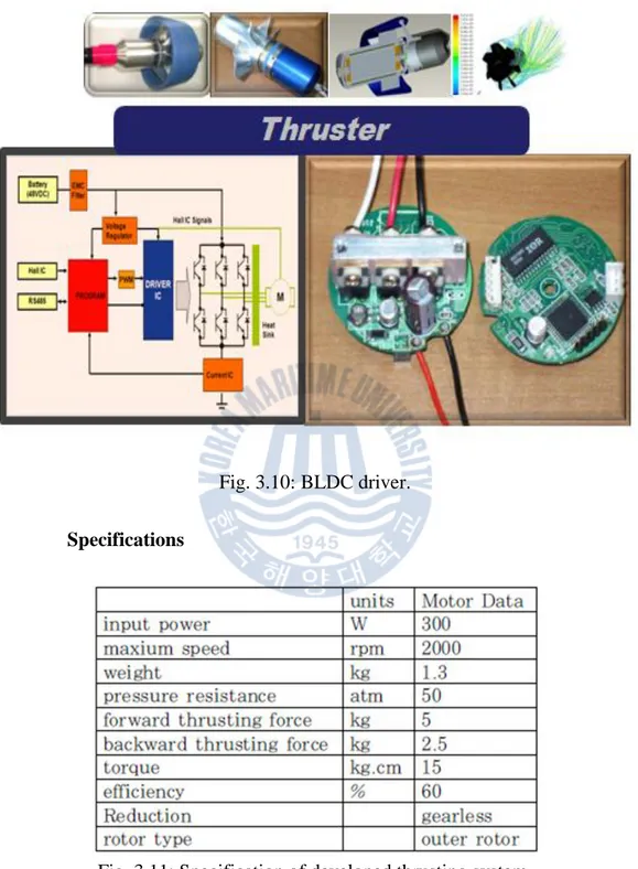
We developed the 300w underwater thrusting system driven by a brushless DC (BLDC) motor for underwater robots. A design of the structure such as the structure analysis on the thrusting system using FEM and the design of the propeller using the fluid analysis has been performed. The performance test of the designed and developed thrusting system in water and in air was undertaken and its results were compared with an existing product with high performance. The comparison results show that the developed thrusting system has better performance by 16% in forward thrusting force and by 12% in backward thrusting force (Table 3.5) [7]. Also, a new structure such as decoupling and non-gear structure has been developed with characteristics in table 3.4.
29
Fig. 3.10: BLDC driver.
Specifications
30 Table 3.4: Comparison with present products.
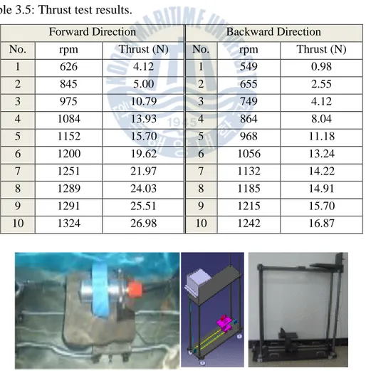
Table 3.5: Thrust test results.
Fig. 3.12: Configuration of experimental apparatus. Division Power transmission
structure
Characteristics
Present products
Motor + Gear + Magnetic coupling
Complex, good sealing, light, small Motor + Magnetic
coupling
Complex
Motor + Gear + sealer Complex, bad sealing Motor + sealer Simple, bad sealing Developed
system
Magnetic outer rotor + can
Simple, good, sealing, heavy
Forward Direction Backward Direction No. rpm Thrust (N) No. rpm Thrust (N)
1 626 4.12 1 549 0.98 2 845 5.00 2 655 2.55 3 975 10.79 3 749 4.12 4 1084 13.93 4 864 8.04 5 1152 15.70 5 968 11.18 6 1200 19.62 6 1056 13.24 7 1251 21.97 7 1132 14.22 8 1289 24.03 8 1185 14.91 9 1291 25.51 9 1215 15.70 10 1324 26.98 10 1242 16.87
31
3.3 Sensor
3.3.1 Model PSH (high performance pressure transducer)
PSH model is high precise and its media-wetted materials are composed of stainless steel 316L, having excellent corrosion-resistant properties. It is applied to precise measurement and builds an inner amplifier to interface with various kinds of controllers.
Applications:
Process control
Hydraulics & Pneumatic Compressor control Chillers Refrigeration equipment Specifications: Range: 0-2 kgF cm / 2 Voltage: 1-5VDC Accuracy: ±0.15%FS
Thermal effect on zero: ±0.03%FS/C Operating temperature range: 0
20 80 C
Weight:140g
Fig. 3.14: Internal circuit diagram of pressure sensor. Fig. 3.13: Model PSH.
32 3.3.2 Developed AHRS
a. Purpose of developing AHRS :
Fields of use in robotics, aerospace, autonomous vehicle, marine industry.
Develop a low-cost system while still keep high accuracy. Initiatively keep technology and develop, integrate into
another applications flexibly.
Fig. 3.15: Attitude heading reference system. Design Attitude heading reference system:
Each method which determines attitude and heading has advantages and disadvantages. The method using rate gyro has good performance in short time but results in drift after long period. Meanwhile, the method using accelerometer has good performance when the body is under non-acceleration state but is invalid when the body is accelerating. The method using magnetometer has no drift but is valid only in the homogeneous and
33
undisturbed Earth’s magnetic field. Therefore, a fusion method is necessary to exploit advantages of each method. [8]
b. Hardware design process
Fig. 3.16: Attitude heading reference system block schematic.
In our approach, the tri-axis inertial sensor with magnetometer ADIS16405 which is a product of Analog Devices, Inc. are used. Signals coming from the sensor are processed by digital signal controller TMS320F28335 where Kalman filter and data fusion algorithm are implemented. A prototype PCB is developing as illustrated in following figure 3.21.
34 ADIS16405 sensor:
The ADIS16405 sensor is a complete inertial system that includes a tri-axis gyroscope, a tri-axis accelerometer, and a tri-axis magnetometer. The ADIS16405 combines industry-leading MEMS technology with signal conditioning that optimizes dynamic performance. This sensor provides a simple, cost-effective method for integrating accurate, multi-axis inertial sensing into industrial systems, especially when compared with the complexity and investment associated with discrete designs. An improved SPI interface and register structure provide faster data collection and configuration control.
Fig. 3.18: Axial Orientation. Specifications:
Fig. 3.19: Functional block diagram.
Tri-axis, digital gyroscope ±75º/sec, ±150º/sec, ±300º/sec
Output noise : 0.9 °/sec Tri-axis, ±18g digital accelerometer
Output noise : 9 mg
Tri-axis, ± 2.5gauss digital magnetometer Output noise : 1.25 mgauss
Digitally controlled sampled rate up to 819.2SPS Operating temperature range: -40ºC to +105ºC
35 Prototype PCB:
The most important element in using kalman Filter is real time. So the collection of microcontroller is necessary to satisfy it. Digital signal controller TMS320F28335 with frequency up to 150MHz is chose. It is connected with sensor through SPI interface, and transfer attitude data to computer by using serial port.
Fig. 3.20: TMS320F28335 pins, SPI port.
36 AHRS’s Interface:
The AHRS’s interface is designed by Visual Studio 2008. It is one of powerful tools for making Graphical Application Programming Interface (API) which is useful, flexible, eye-catching… By using this interface, we can easily setup and supervise the AHRS.
Fig. 3.22: AHRS’s Interface.
c. Control algorithm and experiments:
In first 10 seconds, use Low-Pass filter to get the average Euler Angles with frequency 50Hz. The initial Quaternion of Kalman filter loop is calculated from the average Euler Angles. After every loop cycle, converting Euler Angles from Quaternion, we will have the attitude of body. Kalman filter will be discussed more extensively later in the chapter 4.
37
3.4 UDR System
Fig. 3.23: UDR system diagram.
The UDR control system is built by computer interface which has functions such as UDR action supervision, give control command, set up PID Parameters: Kp, Ki, Kd, draw plots and connect with UDR by using RS485 communication every 100ms.
38
Controller board: control 3 Thrusters_48V by RS485 communication with bandrate 38400bps ,3 DC Motor_24V by DC Motor Driver and RC Motor with baudrate 115200bps
Sensor board: collect the attitude signals through using Kalman Filter: roll (defined from [ 180 ...180 ] 0 0 ), pitch(defined from [ 90 ...90 ] 0 0 ), yaw (defined from [ 180 ...180 ] 0 0 ), linear acceleration accX, accY, accZ, and depth of UDR.
The Controller board will send command and will receive UDR’s attitude signals from sensor board every 30ms. After having data, DSP2812 will apply PID Algorithm to control UDR to desired position, attitude …
39
Chapter 4 Theoretical Background
In this chapter, we will review the theoretical background that are the Attitude and Heading representation, Kalman filter, and Proportional Integral Differential (PID) control.
4.1 Attitude and Heading representation
Fig. 4.1: Reference frames.
Before describing the attitude and heading estimation system, we should agree on how attitude and heading angles are represented. Consider a rigid body rotating and translating in the inertial space. Our aim is to
40
estimate attitude and heading of the rigid body in the inertial space. To do this, three right-handed orthogonal coordinate frames are defined [9]
Navigation frame (frame): It was used as reference frame. The n-frame has its origin at some point in the body where the measurement system is located. With x -axis points North, n y -axis points East and n
n
z -axis points vertical down to the Earth’s centre. It is so called
North-East-Down (NED) frame.
Body frame (b-frame): Moving coordinate frame fixed to the body. With the x -axis (roll) points forward, b y -axis (pitch) points to the b
right and the z -axis (yaw) points downward b
Horizontal frame (h-frame): The b-frame is called the h-frame when their attitude angles are zeros.
Various mathematical representation can be used to define the attitude and heading of a body frame with respect to a reference frame such as: direction cosine matrix, Euler angles, Quaternion.
a) Euler Angles: It is utilized because of its intuitive nature and popularity despite drawback such as singularities. The body-fixed angular velocity vector and the Euler rate vector are related through a transformation matrix J2(2)which is undefined for a pitch angle of 0
90
. The Euler angles is obtained by three successive rotations about different axes, known as Euler angle sequence. Following Euler angle sequence is chosen to transform reference to body frame.
41
Fig. 4.2: Euler angle sequence. Rotate through angle (yaw) about reference z-axis. Rotate through angle (pitch) about reference y-axis. Rotate through angle (roll) about new x-axis.
The three rotations may be expressed mathematically by following three separate direction cosine matrices, respectively:
Rotate about z-axis,
0 0 0 0 1 z c s C s c (4.1)
Rotate about y-axis,
0 0 1 0 0 y c s C s c (4.2)
Rotate about x-axis,
1 0 0 0 0 x C c s s c (4.3)
Thus, a transformation from reference to body axes may be expressed as product of these separate transformation as follows:
b n x y z C C C C c c s c s s c c s s c c s s s c s s s c s c s s c c s c c (4.4)
42
Similarly, the inverse transformation from body to reference axes is given by:
T
T
T
Tn b
b n z y x
C C C C C (4.5) b) Quaternion: An alternative to the Euler angle representation is a
four-parameter method based on unit quaternion. It solve the Euler’s singularity which is undefined for a pitch angle of 0
90 . 3 1 2 3 { | T 1, [ , T T] , } [ , , ]T Q q q q q R and (4.6) 2 1 2 3 cos sin 2 q (4.7)
Where the unit vector
1, 2, 3
T is: T And 1222322 1The rotation matrix transform between the linear velocity vector in the inertial reference frame to the velocity in the body-fixed reference frame can be expressed as: 2 2 2 3 1 2 3 1 3 2 2 2 1 2 3 1 3 2 3 1 2 2 1 3 2 2 3 1 1 2 1 2( ) 2( ) 2( ) ( ) 2( ) 1 2( ) 2( ) 2( ) 2( ) 1 2( ) n b R q (4.8)
43
c) Transformation between Euler Angles and Quaternion:
0 1 2 3 2 2 1 2 0 2 3 1 0 3 1 2 2 2 2 3 2 tan 1 2 sin 2 2 tan 1 2 q q q q a q q a q q q q q q q q a q q
2 2 0 1 2 3 1 2 0 2 3 1 2 2 0 3 1 2 2 3 tan 2 2 ,1 2 sin 2 tan 2 2 ,1 2 a q q q q q q a q q q q a q q q q q q (4.9)d) Transformation between Quaternion and Euler Angles:
0 1 2 3cos / 2 cos / 2 cos / 2 sin / 2 sin / 2 sin / 2
sin / 2 cos / 2 cos / 2 cos / 2 sin / 2 sin / 2
cos / 2 sin / 2 cos / 2 sin / 2 cos / 2 sin / 2
cos / 2 cos / 2 sin / 2 sin / 2 sin / 2 cos / 2
q q q q q (4.10)
4.2 Kalman Filter
The Kalman filter is a set of mathematical equations that provides an efficient computational means to estimate the state of a process, in a way that minimizes the mean of the squared error. The filter is very powerful in several aspects: it supports estimations of past, present and even future states and it can do so even when the precise nature of the modeled system is unknown.[10]
44 The Discrete Kalman Filter Algorithm
Fig. 4.3: The Discrete Kalman Filter Algorithm.
The equations for the Kalman filter fall into two groups: time update equations and measurement update equations. The time update equations are responsible for projecting forward (in time) the current state and error covariance estimates to obtain the a priori estimates for the next time step. The measurement update equations are responsible for the feedback- i.e. for incorporating a new measurement into the a priori estimate to obtain an improved a posteriori estimate.
The time update equations can also be thought of as predictor equations, while the measurement update equations can be thought of as corrector equations.
45
Fig. 4.4: The operation of the Kalman filter.
a) The time update equations projects the state and covariance estimates forward from time step k-1 to step k.
The nxn matrix A in the difference equation (1) of time update equations relates the state at the previous time step k-1 to the state at the current step k, in the absence of either a driving function or process noise.
The nxl matrix B relates the optional control input l
u to the state x.
The process noise covariance Q might change with each time step or measurement.
b) The measurement update:
The first task is to compute the Kalman gain K . k
The next step is to actually measure the process to obtain z and k
46
Then final step is to obtain an a posteriori error covariance estimate via P k
After each time and measurement update pair, the process is repeated with the previous a posteriori estimates used to project or predict the new a priori estimates.
4.3 Proportional Integral Differential (PID) control
PID’s are essentially algorithms which are primary used in control application. These algorithms try to control the output of a system by minimising the difference or error between the setpoint (desired value) & current point (observed value). One of the classic application example of PID control would be the oven thermostat. The thermostat’s primary function would be to maintain a certain temperature within the oven by varying the amount of heat the oven’s heating element could give out in order the maintain the set temperature within the oven.
P – Proportional Control I – Integral Control D – Derivative Control
These three terms are then multiplied by their respective constants and then summed up to give the final PID Control output.
. . .
p i d
d error
PID K error K errordt K
dt
(4.11)p
K : Proportional gain, a tuning parameter.
i
K : Integral gain, a tuning parameter.
d
K : Derivative gain, a tuning parameter.
error= set point – current point.
47
Fig. 4.5: A block diagram of a PID controller.
Table 4.1: PID tuning.
Method Advantages Disadvantages Manual
Tuning
No math required. Online method
Requires experienced personnel
Ziegler-Nichols
Proven method. Online method
Process upset, some trail-and-error, very aggressive tuning.
Software tools
Consistent tuning. Online or offline method. May include valve and sensor
analysis.
Some cost and training involved
a) Manual tuning:
If the system must remain online, one tuning method is to first set K i
and K values to zero. Increase the d Kp until the output of the loop oscillates, then the Kp should set to approximately half of that value for a “quarter amplitude decay” type reponse. Then increase K until any offset is i
48
cause instability. Finally, increase K if required, until the loop is acceptably d
quick to reach its reference after a load disturbance. However, too much K d
will cause excessive response and overshoot. A fast PID loop tuning usually overshoots slightly to reach the setpoint more quickly; however, some systems can’t accept overshoot, in which case an over-damped closed-loop systems is required, which will require a Kp setting significantly less than half that of the Kp setting causing oscillation.
Table 4.2: Effects of increasing a parameter independently. Parameter Rise time Overshoot Settling
time Steady-state error Stability p
K Decrease Increase Small
change Decrease
Degrade
i
K Decrease Increase Increase Decrease Degrade
d K Minor Decrease Minor Decrease Minor Decrease No effect Improve if d K small b) Ziegler-Nichols method:
As in the method above, the K and i K gains are first set to zero. d
The Kp gain is increased until it reaches the ultimate gain, K , at which the u
output of the loop starts to oscillate. K and the oscillation period u P are u
49 Table 4.3: Ziegler-Nichols method.
Control Type Kp K i K d
P 0.5K u
PI 0.45K u 1.2Kp / P u
PID 0.6K u 2Kp / P u Kp P /8 u
c) PID tuning software:
Most modern industrial facilities no longer loops using the manual calculation methods shown above. Instead, PID tuning and loop optimization software are used to ensure consistent results. These software will gather the data, develop process models, and suggest optimal tuning. Some software packages can even develop tuning by gathering data from reference changes.
Advances in automated PID loop tuning software also deliver algorithms for tuning PID loops in a dynamic or Non-Steady State (NSS) scenario. The software will model the dynamics of a process, through a disturbance, and calculate PID control parameter in response.
50
Chapter 5 Experiments and Results
5.1 Developed AHRS
51
Fig. 5.1 represents the flow diagram of AHRS system. Kalman filter needs the initial estimates which are as accurately as possible. Hence in first 10 seconds, just calculate the roll, pitch, yaw angles by using Low-pass filter and then transfer to quaternion from Euler Angles. After that apply Kalman with two steps: Predictor equations and Corrector equations to get the real attitude values.
The below figures will illustrate the attitude experiment results that include Roll, Pitch, Yaw angles before filter and after using Kalman filter. The data will be more accurate, with small error and nearly real signals. It will be better if we use more high-speed microprocessor as well as improve the loop time to 500Hz.
Fig. 5.2: Roll angle without filter (Max Error= 6º).
52
In Fig. 5.2 The output signal of Roll angle without Kalman Filter has many noise with Max Error= 6 degree. That isn’t real value of body attitude. However, after through filter, the signal will be better, Max Error= 0.5 degree, and get approximately real value (Fig. 5.3).
Fig. 5.4: Pitch angle without filter (Max Error= 5º).
Fig. 5.5: Pitch angle after filter (error= 0.6º).
In Fig. 5.4 The output signal of Pitch angle without Kalman Filter has many noise with Max Error= 5 degree. That isn’t real value of body attitude. However, after through filter, the signal will be better, Max Error= 0.6 degree, and get approximately real value (Fig. 5.5).
53
Fig. 5.6: Yaw angle without filter (Max Error= 12º).
Fig. 5.7: Yaw angle after filter (Max Error= 1.5º).
In Fig. 5.6 the output signal of Yaw angle without Kalman Filter has many noise with Max Error= 12 degree. That isn’t real value of body attitude. However, after through filter, the signal will be better, Max Error= 1.5 degree. But it will be drifted by over time and not exactly like initial cases before.
54
5.2 UDR Experiments
5.2.1 Buoyancy
Fig. 5.8: UDR in water-tank.
For making buoyancy force, UDR is attached Styrofoam which will exterminate the UDR mass and always make floating without depth control. The Styrofoam volume is calculated by experiments. Fig. 5.9 and Fig. 5.10 show the result when it is floating in the water-tank with Roll angle, Pitch angle near 0 degree. It is convenient to control tilt, depth, and motion.
55
Fig. 5.10: The Pitch angle.
5.2.2 Tilt and Depth Control
( ) p. i. d.d error
u t K error K errordt K
dt
(5.1)Fig. 5.11: PID for Title and Depth control.
PID Algorithm is used to control Tilt and Depth by three DC motors. This is so complex because DC motors are disposed symmetrically by 120 degrees. There are the interactions between rolling control with pitching control and depth control. With small change of roll angle will effect to pitch angle, depth and vice versa. First, the reference signals are compared with feedback signals which are measured by IMU sensor and depth sensor. After
56
through PID controller, the output vector M will cause UDR quickly reach the desired position, orientation.
Fig. 5.12: Control Depth and keep Roll=Pitch=10 degree. a) Experiment with Roll=Pitch=0 degree
p
K = 4.0; K = 0.2; i K = 0.4 d
Fig. 5.13: Control Title to Roll=Pitch=0 degree with disturbance. Fig 5.13 represents the UDR’s attitude in two cases: not controlled and controlled in the disturbance environment. Without control, UDR maintains the free state with Roll and Pitch angle around 0 degree. Under the effect of disturbances, it will change the state and become unstable, oscillation. To put the system back to steady state before the PID algorithm is applied and it take some seconds.
57
b) Experiment with Roll=Pitch=0 degree, Depth=0.2m
p
K = 4.0; K = 0.2; i K = 0.4 d
Fig. 5.14: Control Roll=Pitch=0 degree, Depth=0.2m with disturbance Fig 5.14 represents the UDR’s attitude in two cases: not controlled and controlled in the disturbance environment. We want to keep system in Roll=Pitch=0 degree and Depth=0.2m. When applied PID algorithm the UDR will quickly reach the desired state and maintain it stabilization. Under the effect of disturbances, the UDR will change the state and become unstable, oscillation. But it only exists in a few seconds and will return to steady state before by effect of the controller.
58
c) Experiment with Roll=Pitch=10 degree, Depth=0.2m
p
K = 4.0; K = 0.2; i K = 0.4 d
Fig. 5.15: Control Roll=Pitch=10 degree, Depth=0.2m with disturbance
Fig 5.15 represents the UDR’s attitude in two cases: not controlled and controlled in the disturbance environment. We want to keep system in Roll=Pitch=10 degree and Depth=0.2m. When applied PID algorithm the UDR will quickly reach the desired state and maintain it stabilization. Under the effect of disturbances, the UDR will change the state and become unstable, oscillation. But it only exists in a few seconds and will return to steady state before by effect of the controller.
59
Chapter 6 Conclusion
In this paper, we designed a new UDR structure which can be less affected by external disturbances and operated swift motion to any direction by robust vector propulsion control scheme. Beside that, the control system is completely built with PID algorithm and Kalman filter. Initial experiments carried out good results about AHRS, buoyancy, depth and tilt test. In the next step, to complete and optimize system we need to add more sensors such as DVL, GPS, USBL for the navigation in the water and the surface. Increase the processing speed by using more high-speed microprocessor or embedded computer that will be easy to calculate and apply the complex algorithms.
60
References
[1] http://en.wikipedia.org/wiki/Main_Page
[2] Justin E. Manley, “Unmanned Surface Vehicles, 15 Years of Development”, Proceedings of Oceans 2008, Quebec City, Canada, Sept.2008.
[3] Robert L. Wernli, ”AUV’S -- THE MATURITY OF THE TECHNOLOGY”, Proceedings of Oceans ’99, MTS/IEEE, Seattle, WA , USA, September 1999.
[4] Roman, C.; Pizarro, O.; Eustice, R.; Singh, H. ,” A new autonomous underwater vehicle for imaging research ”, Proceedings of Oceans 2000, MTS/IEEE, vol 1, pp 153-156, September 2000.
[5] Thor I.Fossen, “Guidance and Control of Ocean Vehicles”, John Wiley & Son, New York , 1994.
[6] www.ti.com, Texas Instrument .Inc.
[7] Tae-Hwan Joung, Han-Il Park, Sang-Young Lee, Moon-An Kim…,” An Verify by Experimental Test for Estimation of Propulsion Performance of the Unmanned Underwater Vehicle ”, Conference Proceedings of Korea Ocean Engineering 2011.
[8] Ngo Thanh Hoan, “A Study on a Low-Cost Attitude and Heading Estimation System for ROVs”, Master thesis, Korea Maritime University, August 2008.
[9] D. H. Titterton, J. L. Weston, “Strapdown Inertial Navigation Technology”, 2nd
edition, American Institute of Aeronautics and Astronautics, 2004.
[10] Greg Welch, Gary Bishop, “An Introduction to the Kalman Filter”, UNC-Chapel Hill, TR 95-041, July 24, 2006
[11] A. J. Baerveldt, R. Klang, “A low-cost and low-weight attitude estimation system for a autonomous helicopter”, in Proc. 1997 IEEE Int. Conf. on Intelligent Engineering Systems, Budapest, Hungary, pp. 391-395, 1997.
[12] D. Jurman, M. Jankovec, R. Kamnik, M. Topic, “Calibration and data fusion solution for the miniature attitude and heading reference system”, Sensors and Actuators, pp. 411-420, 2007.
61
[13] P. Zarchan, H. Musoff, “Fundamentals of kalman filtering: A practical approach”, American Institute of Aeronautics and Astronautics, 2005. [14] B. Barshan, H.F. Durrant-Whyte, “Inertial navigation systems for
mobile robots”, IEEE Transactions on Robotics and Automation, vol.11, no.3, 1995.
[15] US Navy, “The Navy Unmanned Undersea Vehicle (UUV) Master Plan”, November 9, 2004, p.67.
[16] J.Yuh, “Learning Control for Underwater Robotic Vehicles”, IEEE International Conference on Robotics and Automation, Atlanta, GA, May 1993.
[17] Podder, Tarun K., G. Antonelli, and N. Sarkar, “Fault-Accommodating Thruster Force Allocation of an AUV Considering Thruster Redundancy and Saturation”, IEEE Transaction on Robotics and Automation, April 2002. [18] Yasuyuki Kataoka, Kazuma Sekiguchi, MitsujiSampei, “Nonlinear Control and Model Analysis of Trirotor UAV Model”, the 18th IFAC World Congress, Milano (Italy) August 28 - September 2, 2011.
[19] GabrielM. Hoffmann, Huang,H.S.L.W. and Tomlin,C.J. (2007). “Quadrotor helicopter flight dynamics and control:Theory and experiment”. Proc. Of AIAA Guidance, Navigation and Control Conference and Exhibit. [20] Ian C. Rust and H. Harry Asada, ” The Eyeball ROV: Design and Control of a S pherical Underwater Vehicle Steered by an Internal Eccentric Mass”, IEEE International Conference on Robotics and Automation, Shanghai, China, May 9-13, 2011.