Frontal Plane Motion with Pelvis and Waist Joint Rotations in Bipedal Walking

ICCAS2005 June 2-5, KINTEX, Gyeonggi-Do, Korea

Frontal Plane Motion with Pelvis and Waist Joint Rotations in Bipedal Walking

School of Electrical Engineering and Computer Science, Seoul National University, Seoul, Korea (Tel : +82-2-880-7313; Fax: +82-2-885-4459; Email:∗psalm150,∗∗charles34,∗∗∗[email protected])

Abstract: Although the progress in bipedal walking is impressive in recent years, biped robots still require very high torque and can walk only

for a short time interval with their internal batteries. Therefore, further research needs to be carried out to enhance walking efficiency of these robots. In order to achieve this goal, we attempt to imitate human walking with pelvis and waist joint rotations in the frontal plane. In order to investigate the effect of the pelvis and waist joint rotations in the frontal plane motion, we study the frontal plane model with a triangular structure made up of a waist joint and two hip joints. Through simulation, we show that the pelvis rotation can reduce the maximum torque and the control effort, and the waist joint rotation can reduce the trunk sway caused by the pelvis rotation. The combination of these two rotations makes the bipedal walking in the frontal plane more efficient.

Keywords: bipedal walking, frontal plane motion, pelvis and waist joint rotations, maximum torque, control effort

1. Introduction

Many researchers have studied the walking motion of biped robots in order to achieve a stable motion. Although there has been great progress in bipedal walking researches, biped robots still require high torque motors and can walk only for a short time interval with their internal batteries.

Some studies have been conducted to improve the energy efficiency in moving robots. Some of them are the studies on the design of a gait trajectory for walking in a multi-leg robot [1, 2], the trajec-tory generation and the control considering energy efficiency in a one-leg hopping robot [3, 4], the passive walking in a biped robot [5] and the analysis of energy efficiency in a biped robot [6]. How-ever, these studies were only restricted to the walking motion in the sagittal plane.

There have also been studies with respect to the frontal plane mo-tion. These are the control of a multi-link model [7–9], the tra-jectory generation based on the inverted pendulum considering the zero moment point (ZMP) condition [10, 11] and the control based on the symmetric motion and the reinforcement learning [12]. Yet, these studies did not explore the motion in the aspect of energy ef-ficiency.

In order to improve energy efficiency in the frontal plane, we in-vestigate the pelvis joint and waist joint motions in human walking. Humans rotate pelvis and waist joints in order to move the center of gravity (CoG) during walking, and Leeuwen [13] measured the pelvis rotation in human walking. We apply the structure and mo-tion of a human to a biped robot and show that the pelvis rotamo-tion can reduce the maximum torque and control effort in the frontal plane, and the waist joint rotation can reduce the trunk sway.

2. Biped robot model

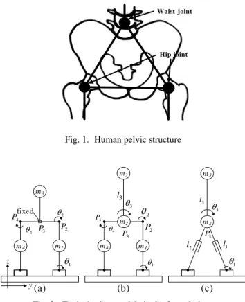
The pelvis of a human has a triangular structure as shown in Fig. 1. However, the typical robot models in the frontal plane motion, which is to move its CoG, can be classified into three types as shown in Fig. 2. In motions generated by these models, it is difficult to show that the pelvis and waist joint rotations can improve energy efficiency. In Fig. 2(a), there is no waist joint rotation. In Fig. 2(b), the distance between the waist joint and the hip joint along z-axis is zero. When walking with the hip rotation is realized in this model, hip joint torque is very large at early stage of the hip rotation. Fig.

Waist joint

Hip joint

Fig. 1. Human pelvic structure

m3 m1 m4 1 θ 2 θ 3 θ 2 l 3 l 3 P P2 4 θ 4 P m3 3 θ 3 l m2 3 P 1 l m2 m3 y z m1 m4 1 θ 2 θ 3 P P2 4 θ 4 P (a) (b) (c) 1 θ fixed

Fig. 2. Typical robot models in the frontal plane

2(c) shows a frontal plane model in which the hip and waist joints are collocated like a model in the sagittal plane. Since the waist joint, pelvis and trunk rotations are not separable, it is difficult to show how the energy efficiency is affected by the pelvis rotation in this model.

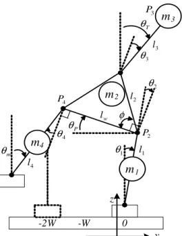
In order to study the effect of pelvis and waist joint rotations in walking, we propose a frontal robot model as shown in Fig. 3. The triangular pelvis is made of a waist joint and two hip joints, which is similar to a human pelvis (Fig. 1). In Fig. 3, θ1is the rotation angle

of the ankle joint, θ2is the rotation angle of the hip joint connected

to the supporting leg, θ3is the rotation angle of the waist joint, θ4

is the rotation angle of the hip joint connected to the moving leg,

lwis the distance between two hip joints, and W is the half of lw.

The rotation angle θP of pelvis, with respect to the horizontal line 2248

y z 0 -W

m

θ

θ

θ

φ

m

θ

m

m

θ

Fig. 3. Robot model with the triangular pelvis in the frontal plane Table 1. Model parameters

Parameter Value Parameter Value

l1 0.25m m2 0.4kg lw 0.09m m3 1kg l3 0.2m m4 1.8kg m1 1.8kg φ 60◦ S 0.06m T 1.0s Lf 0.12m Wf 0.08m W 0.045m

is also shown in Fig. 3. The values of these parameter are shown in Table 1 which are obtained based on the robot in our laboratory. In Table 1, S is the step size, Lfand Wfare the length and width of a

foot, respectively. From the kinematics of a biped robot, the center of gravity (yCoG, zCoG) in the y and z directions are expressed as

(yCoG, zCoG) = 1 m1+ m2+ m3+ m4(¯yCoG, ¯zCoG), ¯ yCoG = (0.5m1+ m2+ m3+ m4)l1sinθ1 −(0.5m2+ m3)l2cos(θ1+ φ + θ2) +m3l3sin(θ1+ θ2+ θ3) −(0.5m2+ 2m4)l2cosφcos(θ1+ θ2) −0.5m4l1sin(θ1+ θ2+ θ4), ¯ zCoG = (0.5m1+ m2+ m3+ m4)l1cosθ1 +(0.5m2+ m3)l2sin(θ1+ φ + θ2) +m3l3cos(θ1+ θ2+ θ3) +(0.5m2+ 2m4)l2cosφsin(θ1+ θ2) −0.5m4l1cos(θ1+ θ2+ θ4).

In order to determine θ4 in Fig. 3, let us consider θmwhich is the

angle between a moving foot and the z-axis. The torque applied to the moving foot increases as θmincreases. When θmis smaller than θ1, the torque is reduced but the foot is more likely to collide with

CoG l CoG θ

m

m

m

m

m

Fig. 4. Inverted pendulum model for the frontal plane motion

the other foot. Since the distance between two legs in the model is small, we set θmto be equal to θ1 in order to avoid possible

collision. Therefore, θ4must satisfy θ4 = −θ2. Then, the CoG in

the above is simplified as ¯ yCoG = (0.5m1+ m2+ m3+ 0.5m4)l1sinθ1 −(0.5m2+ m3)l2cos(θ1+ φ + θ2) +m3l3sin(θ1+ θ2+ θ3) −(0.5m2+ 2m4)l2cosφcos(θ1+ θ2), ¯ zCoG = (0.5m1+ m2+ m3+ 0.5m4)l1cosθ1 +(0.5m2+ m3)l2sin(θ1+ φ + θ2) +m3l3cos(θ1+ θ2+ θ3) +(0.5m2+ 2m4)l2cosφsin(θ1+ θ2). (1)

Typically, a biped robot moves its CoG in the frontal plane by ro-tating its ankle joint, and keeps its trunk upright by roro-tating its hip joint. There is no need to rotate the waist joint, so the pelvis does not rotate, i.e., θP=0. In the walking motion that we are gong to

study, the ankle joint and hip joints are rotated to move its CoG while the waist joint is rotated to keep the trunk upright. In this walking motion, the pelvis is rotated, i.e., θP 6=0.

3. Frontal plane motion

3.1. Frontal plane motion at the Cartesian coordinate

It is difficult to get a joint trajectory directly from a ZMP trajectory when a multi-linked robot walks. In order to generate a joint tra-jectory, we need to investigate a simple motion with the ZMP into consideration. So we generate a trajectory of CoG in the frontal plane using an inverted pendulum model (Fig. 4). In the single sup-port phase, the rotational axis of the ankle joint of the supsup-porting foot corresponds to the rotational axis of the inverted pendulum, and the torque applied to the ankle joint can be considered as the external torque of the inverted pendulum. Since ZMP is expressed proportionally to the torque applied to the ankle joint in walking, it becomes the center of the supporting foot when the torque applied to the ankle joint is zero. Similarly, when the external torque in the inverted pendulum is zero, ZMP is at the rotational axis of the in-verted pendulum. This means that the trajectory of the CoG of a

Case A1 Case B1 1 θ 2 θ 3 θ Case C Case A2 Case A3 Case B2 Case B3 1 θ θ1 1 θ θ1 θ1 1 θ 3 θ 3 θ 3 θ 2 θ 2 θ 2 θ θ₂

Fig. 5. Seven types of the frontal plane motion

robot is equal to the trajectory of the CoG of the inverted pendulum moving under the gravity field without external torque.

In the inverted pendulum model as shown in Fig. 4, the dynamic equation is

cmCoGl2CoGθ¨CoG− mCoGglCoGsinθCoG= τ, lCoGsinθCoG= yCoG.

If the inverted pendulum moves under the gravity field without ex-ternal torque and θCoGis small, the equation is simplified as

lCoGy¨CoG= gyCoG.

And its solution is

yCoG(t) = −W cosh( q g l_CoGt) + q lCoG

g ˙yCoG(0)sinh( q

g lCoGt).

(2)

As the motion is reversed in the middle of a walking period T , the trajectory of CoG must satisfy the following constraint:

˙yCoG(T₂) = 0. (3)

From Eq. (3), the initial velocity for walking is derived as

˙yCoG(0) = − r g lCoG W 1 − exp(q g l_CoGT ) 1 + exp(q_l g CoGT ) .

3.2. Seven types of frontal plane motion at the joint coordinate

There are many solutions for the joint trajectories which can be de-rived from Eq. (2) of CoG in the frontal plane. In order to represent the typical walking motion well while using as small number of pa-rameters as possible, we only consider the trajectory in which the joint angles in Eq. (1) satisfy the following relations:

θi= wiθ, (i = 1, 2, 3).

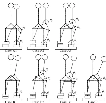
We select seven types of motion to investigate the effect of the pelvis and waist joint rotations (Fig. 5). Using the parameters (w1, w2,

w3), the seven types of motions in Fig. 5 are represented as A1:(1,-1,0), A2:(1,0,-1), A3:(1,1,-2), B1:(1,0,0), B2:(1,1,-1), B3:(1,-1,1) and C:(1,1,0). The trunk is kept in the upright position in the cases Ai (i=1,2,3), sways slightly in the cases Bi (i=1,2,3), and sways dramatically in the case C. A1 is the typical movement of CoG of biped robots, in which the pelvis and waist joints do not rotate and the trunk is kept upright. Most of robots move their CoG based on this kind of motions for walking. In the case A2, the pelvis is rotated by the ankle joint and the trunk sways by the pelvis rotation is compensated entirely by the waist joint rotation in order to keep the trunk upright. In the case A3, the pelvis is rotated by the ankle and hip joints and the sway of the trunk is compensated completely by the waist joint rotation. In the case B1, the pelvis is rotated by the ankle joint and the trunk sways since the waist joint does not rotate. In the case B2, the pelvis is rotated by the ankle and hip joints as in the case A3 but the trunk sways slightly since the sway of the trunk is compensated partially. In the case B3, the pelvis does not rotate as in the case A1 but the trunk sways slightly since the waist joint rotation is utilized not to compensate the sway of the trunk but to move the CoG of the robot. In the case C, the pelvis is rotated by the ankle and hip joints and the trunk sways dramatically.

The trajectory generated by rotating only the hip joint requires the hip joint to rotate over 60 degrees. But the hip joint can rotate only up to 30 degrees because of the structural limitation in the robot we have. Therefore, we exclude the trajectory of the CoG generated by rotating only the hip joint.

4. Simulation

4.1. Measure of performance

To compare the performance of each type of motion, we utilize four measures, i.e., ZMP, control effort, the maximum torque and the angle of the trunk θT as shown in Fig. 3. The angle of the trunk

indicates the extent of the trunk sway. ZMP is used only to make sure that the robot does not fall down.

1. ZMP : ZMP is calculated by the force distribution at the sup-porting foot as follows [14]

xZM P = Pn i=1xifi P_n i=1fi , yZM P = Pn i=1yifi P_n i=1fi .

Here, fiis the reaction force at a point (xi, yi) in the supporting

foot. In order to walk stably without falling down, ZMP must satisfy the following condition:

|xZM P− xf| < 0.5Lf, |yZM P− yf| < 0.5Wf,

where (xf , yf) is the position of the supporting foot, and Lf

and Wf are the length and width of the foot respectively.

2. Control effort : Since a multi-linked robot consumes energy even when its motors do not move, the energy efficiency of bipedal walking should be dealt with in terms of the torque con-sumed by each motor and not in terms of kinetic and potential energies. We compute the control effort as the sum of torques produced by all the motors in a robot [15], i.e.,

C(tf) = (tf− ti)−1 Z _t f ti ||τ ||dt, τ = (τ1, τ2, τ3, τ4). 2250

Ks Kd Ks Kd Ks Kd Ks Kd z y x Kd Kd Kd Kd Kd Kd Kd Kd

Fig. 6. Spring-damper model between the foot and the ground

Here, τiis the torque produced by the i-th motor, which moves

the i-th joint. We must reduce the control effort in order for a robot to walk efficiently.

3. Maximum torque :

τmax= max(τ1, τ2, τ3, τ4).

Since the maximum torque is a factor that can limit the motions of a robot, we should always keep eye on the maximum torque required in generating a trajectory. Even though there is a tra-jectory which is more energy efficient, it is meaningless if it requires very high torque beyond the capability of a motor. The torque required should be lower than the maximum torque that can be generated by a motor, which means that we should keep the maximum torque required as low as possible in generating a walking trajectory.

4. Trunk angle (θT) : We use the angle of the trunk to show the

extent of the trunk sway. Usually, a biped robot has its control system and a battery in the trunk, and manipulates arms con-nected to the trunk. Since the trunk motion is limited by these structures, we should keep eye on the trunk sway.

4.2. Sagittal plane motion and Contact model

For the simulation of forward walking, the sagittal plane motion is needed. We use the trajectory generation method in [17] for the sagittal plane motion.

We use the spring-damper model as shown in Fig. 6 to describe the contact motion between the robot foot and the ground. In this model, we use springs and dampers to compute the reaction force by the ground in the z direction and use only dampers to make friction at the x and y directions. We set the spring coefficient (Ks) to 106 N/m and the damping coefficient (Kd) to 103kg/s.

4.3. Simulation result

During the first four seconds in each simulation time of ten seconds, the initial pose and velocity of each robot joint are adjusted so that the robot is in an appropriate initial condition suitable for the walk-ing trajectory, and the robot start to walk. Each step takes a second and the robot walks six steps in each simulation.

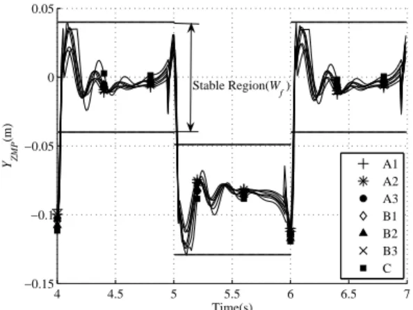
The trajectories of the ZMP for walking are shown in Fig. 7 and Fig. 8. For every frontal plane motions, ZMP remains within the stable region of the supporting foot and those trajectories are similar with each other. However, each ZMP trajectory is not equal to the reference ZMP trajectory, which is designed to be kept the middle of the stable region as shown in Fig. 7 and Fig. 8. We observe over-shoots in YZM Pat the start and at the end of each shift of CoG, and

4 4.5 5 5.5 6 6.5 7 −0.15 −0.1 −0.05 0 0.05 Time(s) YZMP (m) A1 A2 A3 B1 B2 B3 C Stable Region(W f )

Fig. 7. YZM Pin the frontal plane

4 4.5 5 5.5 6 6.5 7 0 0.05 0.1 0.15 0.2 0.25 Time(s) XZMP (m) A1 A2 A3 B1 B2 B3 C Stable Region(L f ) S

Fig. 8. XZM P in the sagittal plane

it converges to the middle of the foot with oscillating in the middle of each shift. In addition, there are overshoots in XZM Pat the start

and at the end of each shift and XZM P increases gradually with

time in the middle of each shift. These overshoots are caused by the force generated by the contact between the foot and the ground dur-ing walkdur-ing. The overshoot of YZM Pis observed to be larger than

that of XZM P since YZM Pis not compensated by a trunk motion.

The increase of XZM P with time between shifts is caused by the

modeling error in the sagittal plane. For the four-mass model in the sagittal plane, the movement of the knee is not considered since the four-mass model is a simplified model that ignores knee joints. Table 2 shows the maximum rotation angle of the pelvis θP,max,

Table 2. Maximum values in the frontal plane

Case θP,max(◦) θT,max(◦) θmax(◦) τmax(N m)

A1 0.12 0.12 11.61 2.67 A2 10.40 0.14 10.45 2.45 A3 18.51 0.13 18.56 2.24 B1 8.86 8.86 8.89 2.11 B2 16.08 8.02 8.07 1.99 B3 0.19 9.67 9.70 2.25 C 14.22 14.22 7.14 1.87 2251

4 4.5 5 5.5 6 6.5 7 0 0.5 1 1.5 2 2.5 3 Time(s) Torque(Nm) A1 A2 A3 B1 B2 B3 C

Fig. 9. Torque applied to the hip joints

4 4.5 5 5.5 6 6.5 7 0.8 1 1.2 1.4 1.6 1.8 2 2.2 2.4 2.6 Time(s)

Control effort in frontal plane(Nm)

A1 A2 A3 B1 B2 B3 C

Fig. 10. Control effort in the frontal plane

the maximum rotation angle of the trunk θT,max, the maximum

rotation angle θmaxand the maximum torque τmaxamong all the

joints for various types of walking in Fig. 5. θP,maxincreases as

the hip joint rotates in order to move the CoG (i.e. in the order of A1, A2 and A3) and increases as the waist joint rotates in order to compensate for the sway of the trunk (i.e. in the order of B3, B1 and B2). θT,maxdecreases as the waist joint rotates, otherwise it

is equal to θP,max. In the case B3, the waist joint rotates in order

to move the CoG, and the trunk rotates even though the pelvis does not rotate.

θmaxcan be minimized by using all the joints for moving the CoG.

As the number of joints used to move the CoG decreases, the ro-tation angle of each joint increases, and the trunk sway decreases. When we have to compensate a large sway of the trunk, θmax

ap-peares at the waist joint because the sway is compensated only by the waist joint. If the motor of the waist joint can not rotate fast enough, the robot will walk slowly.

When all the joints are used in order to move the CoG, τmax

ap-pears at the motor of the hip joint. Figure 9 shows the torque of hip joint during walking. Comparing τmax’s in the cases A1, A2

and A3 in which the trunk did not sway, we can know that τmax

decreases with increasing the angle of the pelvis rotation. In addi-tion, comparing τmax’s in the cases B1, B2 and B3 in which the

trunk sways about 8∼9 degrees, we can see that the pelvis rotation reduces τmax. τmaxis 2.67Nm in the case A1, in which the trunk

4 4.5 5 5.5 6 6.5 7 1.8 2 2.2 2.4 2.6 2.8 3 Time(s)

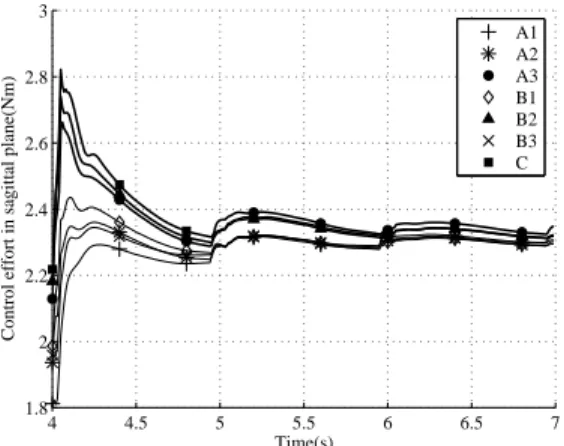
Control effort in sagittal plane(Nm)

A1 A2 A3 B1 B2 B3 C

Fig. 11. Control effort in the sagittal plane

4 4.5 5 5.5 6 6.5 7 2 2.5 3 3.5 Time(s)

Total control effort(Nm)

A1 A2 A3 B1 B2 B3 C

Fig. 12. Total control effort

doesn’t sway and the pelvis doesn’t rotate, and it decreases about 0.022Nm per degree of the pelvis rotation. In the case of B3, in which the trunk sways about 8∼9 degrees but the pelvis doesn’t ro-tate, τmaxis 2.25Nm, and it decreases about 0.016Nm per degree

of the pelvis rotation. In the case of C, in which the trunk sways about 14 degrees and the pelvis rotates, τmaxis 1.87Nm.

Figure 10 shows the control effort in the frontal plane from ti=4s

to tf=7s. Comparing the control efforts in the frontal plane for all

cases, we can find that the pelvis rotation reduces the control effort. Without the constraint requiring that the trunk must be kept upright, we can find that the motion in the case C is the most efficient. In the case C, the control effort is reduced by about 28% compared to that in the case A1, which is the typical type of motion for most biped robots.

Figure 11 shows the control effort in the sagittal plane, and Fig. 12 shows the total control effort. From these figures, we can see that the control effort in the sagittal plane is slightly influenced by the frontal plane motion. The total control effort is reduced by about 14% in the case C compared to A1.

In the case C, the maximum torque and the control effort are smaller than any other cases, but the trunk sways dramatically. When there is a limitation in the rotation of the trunk, the robot may still walk efficiently using the motion in the case B2, in which the pelvis ro-tates to move the CoG and the waist joint compensates the trunk sway partially. If the trunk must be kept upright, the robot can walk

efficiently using the motion in the case A3, in which the pelvis ro-tates to move the CoG and the waist joint compensates the trunk sway completely. Depending on the requirements such as the al-lowable trunk rotation, the maximum torque and the control effort, one can choose a suitable type of motion in the frontal plane.

5. Conclusion

In bipedal walking, most robots move their CoG without the pelvis rotation as shown in the case A1. The bipedal walking without the pelvis rotation requires higher maximum torque and larger control effort. If the pelvis rotation is added to this motion, the maximum torque and the control effort in the frontal plane can be reduced. Furthermore, the trunk sway due to the pelvis rotation can be re-duced by adding the waist joint rotation. Though the waist joint ro-tation increases the maximum torque and the control effort slightly, these are still smaller than their counterparts in the case where there is no pelvis rotation. A robot can walk efficiently utilizing only the pelvis rotation when there is no need to keep the trunk upright. When there is a need to reduce the sway of the trunk, a robot can still walk efficiently utilizing the pelvis and waist joint rotations.

References

[1] Ryo Kurazume, Ahn Byong-won, Kazuhiko Ohta, Tsutomu Hasegawa, “Experimental study on Energy Efficiency for Quadruped Walking Vehicles,” IEEE/RSJ International

Con-ference on Intelligent Robots and Systems(IROS), pp.

613-618, Oct. 2003.

[2] Duane W. Marhefka, David E. Orin, “Gait Planning for En-ergy Efficiency in Walking Machines,” IEEE International

Conference on Robotics and Automation(ICRA), pp. 474-480,

April 1997.

[3] R. Dummer, M. Berkermeier, “Low-Energy Control of a One-legged Robot with 2 Degrees of Freedom,” IEEE International

Conference on Robotics and Automation(ICRA), pp.

2815-2821, April 2000.

[4] Evangelos Papadopoulos, Nicholas Cherouvim, “On Increas-ing Energy Autonomy for a One-Legged HoppIncreas-ing Robot,”

IEEE International Conference on Robotics and Automa-tion(ICRA), pp. 4645-4650, April 2004.

[5] Mariano Garcia, Anindya Chatterjee, Andy Ruina, “Speed, Efficiency, and Stability of Small-Slope 2-D Passive Dy-namic Bipedal Walking,” IEEE International Conference on

Robotics and Automation(ICRA), pp. 2351-2356, May 1998.

[6] Filipe M. Silva, J.A. Tenreiro Machado, “Energy Analysis During Biped Walking,” IEEE International Conference on

Robotics and Automation(ICRA), pp. 59-64, May 1999.

[7] R.E. Goddard Jr., H. Hemani and F.C. Weimer, “Biped side step in the frontal plane,” IEEE Transactions on Automatic

Control, Vol. AC-28, No. 2, pp. 179-186, Feb. 1983.

[8] H. Hemani and B.F. Wyman, “Modeling and control of con-strained dynamic systems with application to biped locomo-tion in the frontal plane,” IEEE Transaclocomo-tions on Automatic

Control, Vol. AC024, No. 4, pp. 526-535, Aug. 1979.

[9] K. Iqbal, H. Hemani and S. Simon, “Stability and control of a frontal four-link biped system,” IEEE Transactions on

Biomedical Engineering, Vol. 40, No. 10, pp. 1007-1017, Oct.

1993.

[10] Philippe Sardain, Mostafa Rostami and Guy Bessonnet, “An Anthropomorphic Biped Robot: Dynamic Concepts and Tech-nological Design,” IEEE Transactions on Systems, Man, and

Cybernetics-Part A: Systems and Human, Vol. 28, No. 6, Nov.

1998.

[11] T. Furuta, T. Tawara, Y. Okumura, M. Shimizu, K. Tomiyama, “Design and construction of a series of compact humanoid robots and development of biped walk control strategies,”

Robotics and Autonomous Systems, Vol. 37, pp. 81-100, Nov.

2001.

[12] Chee-Meng Chew and Gill A. Pratt, “Frontal plane algorithms for dynamic bipedal walking,” Robotica, Vol. 22, pp. 29-39, Jan. 2004.

[13] J.L. Van Leeuwen, P. Vink, C.W. Spoor, W.C. Deegenaars, H. Fraterman and A.J. Verbout, “A Technique for Measure-ing Pelvic Rotations DurMeasure-ing WalkMeasure-ing on a Treadmill,” IEEE

Transactions on Biomedical Engineering, Vol. 35, No. 6, pp.

485-488, June 1988.

[14] Atsushi Konno, Noriyoshi Kato, Satoshi Shirata, Tomoyuki Furuta, Masaru Uchiyama, “Development of a Light-Weight Biped Humanoid Robot,” IEEE/RSJ IROS2000, vol. 3, page(s) 1565-1570, Oct.-Nov. 2000.

[15] Junggon Kim, Jonghyun Baek, F. C. Park, “Newton-type al-gorithms for robot motion optimization,” IEEE/RSJ

Interna-tional Conference on Intelligent Robots and Systems, vol. 3

pp. 1842-1847, Oct. 1999.

[16] Jong H. Park, Yong K. Rhee, “ZMP Trajectory Generation for Reduced Trunk Motions of Biped Robots,” IEEE/RSJ

Inter-national Conference on Intelligent Robots and Systems, pp.

90-95, Oct. 1998.

[17] Jong H. Park, “Impedance Control for Biped Robot Locomo-tion,” IEEE Transactions on Robotics and Automation, Vol. 17, No. 6, Dec. 2001.