Estimation of Non-Gaussian Probability Density by Dynamic Bayesian Networks

1. INTRODUCTION

Probability estimation is an important issue for many engineering applications, especially, for pattern recognition, signal detection, artificial intelligence, etc. Several parametric and nonparametric techniques are available for the estimation [1]. Parametric methods are the simplest to estimate the parameters of a distribution of known form. A Gaussian distribution is widely used as a parametric density model due to its convenient statistical analysis. However, non-Gaussian distributions are often encountered in practical applications. A nonparametric method is more important to this case for which the form of the distribution is unknown. The histogram is the simplest nonparametric approach available. However, the method is less attractive because of its discontinuous nature and because it requires a large amount of data. Another popular nonparametric method is the kernel-based approach in which an estimator is constructed using a set of kernel functions. The best known kernel-based approach is the Parzen-window estimate [2] which uses Gausssian kernels. For the best performance, an appropriate kernel function and its parameter values are chosen for specific data samples. However, the method is very sensitive to parameter values and it is often difficult to determine the optimal kernel. Additional computation, such as smoothing, is sometimes needed.

In recent years, several approaches to PDF estimation have been proposed, such as soft computation, machine learning, information theory, etc. In [3], Fiori and Bucciarelli proposed estimating the distribution of a quasi-stationary random process by using an adaptive neural network which was trained to maximize the differential entropy. M. Srikanth et al. utilized a MinMax measure to estimate a distribution, which is a quantitative measure of information contained in a given set of moment constraints [4]. A conditional

distribution function (CDF) estimate was developed by A. Sarajedini et al. in [5] based on sigmoidal network learning and compared to a kernel CDF estimator for a higher dimensional problem. Miller and Horn investigated estimating both a PDF and CDF by using an information-based learning in which encoding and decoding steps were proposed [6]. A generalized Gaussian distribution was involved in [7] where an estimate of a PDF shape parameter was addressed. In [8], Modha and Fainman obtained a PDF estimate using an exponential family based on multilayer feedforward networks, and derived an unsupervised learning algorithm for ML function. Baram and Roth developed an estimation method that maximized the output entropy of a sigmoidal neural network and named the proposed approach density shaping [9].

We propose a new probability model estimation approach for discrete problems using a DBN and a set of kernel functions. A Bayesian network (BN) is a graphical reasoning system that uses a probability distribution to describe stochastic relationships between its nodes. Each node in a BN represents a random variable and edges indicate dependencies between nodes. A DBN is a dynamic extension of a BN based on an evolving probabilistic model. BNs and DBNs are typically used to solve problems with significant uncertainty.

The proposed approach utilizes a DBN in which a transition distribution is replaced with a set of kernel functions and the probability of feasible variables is expressed in terms of prior probabilities. The optimal parameter values in the estimator are determined via a learning algorithm that maximizes the likelihood function using gradient descent optimization. We test the proposed approach using computer simulations that estimate a discrete-type Poisson density then a nonlinear transformation of the discrete Poisson data.

We next review kernel-based PDF estimation and the Estimation of Non-Gaussian Probability Density by Dynamic Bayesian Networks

Hyun C. Cho*_{, Sami M. Fadali}**_{, and Kwon S. Lee}***

* _{Electrical Engineering Dept./260, University of Nevada-Reno, NV, 89557, USA} (Tel: 1-775-324-2509, E-mail: [email protected])

** _{Electrical Engineering Dept./260, University of Nevada-Reno, NV, 89557, USA} (Tel: 1-775-784-6951, E-mail: [email protected]

*** _{Division of Electrical, Electronic, and Computer Eng., Dong-A Univ., Busan, 604-714, Korea} (Tel: +82-51-200-7739, E-mail: [email protected])

Abstract: A new methodology for discrete non-Gaussian probability density estimation is investigated in this paper based on a dynamic Bayesian network (DBN) and kernel functions. The estimator consists of a DBN in which the transition distribution is represented with kernel functions. The estimator parameters are determined through a recursive learning algorithm according to the maximum likelihood (ML) scheme. A discrete-type Poisson distribution is generated in a simulation experiment to evaluate the proposed method. In addition, an unknown probability density generated by nonlinear transformation of a Poisson random variable is simulated. Computer simulations numerically demonstrate that the method successfully estimates the unknown probability distribution function (PDF).

DBN. Then we describe our proposed estimation approach and derive its learning algorithm. Finally, we

present and discuss our simulation results. j k j k j

J t t β η β β ∂ ∂ + = +1) ( ) ( ₍₇₎

2. KERNEL-BASED PROBABILTY ESTIMATE where tk is discrete time, η is the learning rate. We

expand the partial differential equations using the chain rule as

A kernel-based estimate is typically composed of a mixture of kernel (basis) functions

) , ( ) ( 1 ) ( ) ( j j i N j i i j i i j x x x P x P x P J J β φ α α − = ∂ ∂ ∂ ∂ = ∂ ∂

∑

≠ (8)

∑

= − = N i i i i x x x P 1 ) , ( ) ( αφ β ₍₁₎

where x is a data vector, P(x) is the probability of x, φ is a kernel function, and αi and βi are parameters. Based

on probability axioms, the kernel function must satisfy φ ≥ 0 and the parameters αI must be positive.

and         ∂ − ∂ = ∂ ∂ ∂ ∂ = ∂ ∂

∑

≠ j j j i j n j i i j i i j x x x P x P x P J J β β φ α β β ) , ( ) ( 1 ) ( ) ( (9) 1 ) ( =

∫

φ udu (2)

The parameter values are determined using the recursions (6) and (7) with the derivatives expressed as (8) and (9).

The parameters αi and βi affect estimation performance.

Thus, choosing the parameter values is one of crucial issues in probability estimation. A natural method for choosing the parameters is to plot several curves with different values and visually examine them to search for the best fit. However, numerous applications require an automated or an adaptive optimization approach.

3. DYNAMIC BAYESIAN NETWORKS A BN is a graphic model for stochastic relationships. It represents random variables as nodes and their dependencies as edges between the nodes. The random variables are assumed to have a finite number of states. The BN is described by a directed acyclic graph and a table of conditional probabilities. Let U = (A, B, C, D) be a universe of random variables, then a corresponding BN is depicted in Fig. 1.

ML estimation [10] is used to determine the optimal parameter values in (1). Assuming independent data points, the objective function is defined as

∏

= = N i i o x P x L 1 ) ( ) , | ( α β (3)

A

C

D

B

Applying the natural logarithm to (3), we get

∑ ∑

∑

= = =         − = = = N i N j j j i j N i i o x x x P L x L 1 1 1 ) , ( ln ) ( ln ) ln( ) , | ( β φ α β α (4) Fig. 1. An example of a BN.

We maximize (4) to obtain two parameter vectors

[

]

T N α α α α= _{1 2 L} and

[

T N β β β β= _{1 2 L}

]

In this network, the probabilities P(A), P(B), P(C|A), and P(D|A,B) must be known. A joint probability P(U) is calculated as ) , | ( ) | ( ) ( ) ( ) , , , ( ) ( B A D P A C P B P A P D C B A P U P = = (10)

∑ ∑

= =         − = N i N j j j i j x x J 1 1 , ln ( , ) max α φ β β α (5)

By gradient descent method, the update rules for the

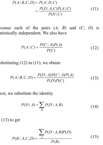
parameters are expressed as Inference is the task of calculating the probability of _{each node by probability calculus from other} probabilities. For instance, in Fig. 1, conditional probability of the variable A given B, C, and D is expressed using Bayes rule as

j k j k j J t a t α η α ∂ ∂ + = +1) ( ) ( ₍₆₎ and

where the conditional probability P(xk|xk-1) is called the

transition probability. A higher-order Markov model provides a more sophisticated solution but at an increasingly higher computational cost. A hidden Markov model (HMM) is a popular structure in which an observation variable depends on a hidden state and a sequence of hidden states evolves according to a Markov process. Fig. 3 illustrates a typical example of an HMM. ) | ( ) | ( ) , | ( ) , | ( ) , , | ( C D P C A P C A D P C D A P D C B A P = = (11)

because each of the pairs (A, B) and (C, D) is statistically independent. We also have

) ( ) ( ) | ( ) | ( C P A P A C P C A P = (12) x₁ x₂

...

x_T y₁ y₂ y_T Substituting (12) in (11), we obtain ) ( ) ( ) ( ) | ( ) | ( ) , , | ( C P D P A P A C P A D P D C B A P = ₍₁₃₎ Fig. 3. An example of HMM. Next, we substitute the identity

The joint probability of the hidden states and observation variables is expressed similarly to the first Markov model as

∑

= B B A D P A D P( | ) ( | , ) ₍₁₄₎ in (13) to get

_∏

= − = T k k k k k k k y P y P y x Px x P y x x P 2 1 1 1 1) ( | ) ( | ) ( | ) ( }) , ({ ₍₁₇₎ ) ( ) ( ) , | ( ) , , | ( B P D P B A D P D C A B

P ₌

∑

A (15) _{where the state transition probability P(x}

k|xk-1) is formed

by a single transition matrix for a time-invariant HMM. The observation probability P(yk|xk) is usually modeled

as Gaussian, a combination of Gaussians, or a neural network. In (17), the transition state xk and observation

state yk are decomposed into deterministic and

stochastic terms as This BN illustrates a quit simple computation of

probability for a particular set of random variables. However, in case of complicated or large Bayesian networks, an efficient inference algorithm is required for a probability updating [11].

k k k k k k k k v x g y w x f x + = + = ₋ ) ( ) ( ₁ (18) DBNs are used to model dynamic events and

represents temporally probabilistic relationships among random variables. This temporal (dynamic) aspect of modeling is more realistic in practice such as artificial intelligence, diagnosis, economic analysis, etc. Several DBN models have been proposed for a variety of applications. The simplest DBN example is the first-order Markov model shown in Fig. 2.

where wk and vk are random noise vectors, and f and g

are transition and observation functions, respectively. If both functions are linear and time-invariant, we have the dynamic linear time-invariant model

k k k k k k v x y w x x + = + = ₋ C A 1 (19) x₁ x₂

...

x_T

where A is the state transition matrix and C is the observation matrix. If the two noise vectors in (19) are modeled as zero-mean Gaussian with covariance matrices Q and R, respectively, the transition and observation probabilities are

Fig. 2. A first-order Markov model.

In Fig. 2, a state vector x∈{x1, x2, …, xT} is modeled at

a certain discrete time k∈{1,…, T}. Each variable is assumed to be first order Markov, i.e. it is dependent only upon the variable at the preceding time. A joint probability for this data sequence is expressed as

) R , C ( ~ ) | ( ) Q , A ( ~ ) | ( _{1 1} k k k k k k x N x y P x N x x P _{− −} (20)

∏

= − = T k k k T P x P x x x x x P 2 1 1 2 1, ,..., ) ( ) ( | )

( (16) _{where N(⋅) denotes Gaussian.}

After constructing the Bayesian network, a learning procedure is developed, based on given data samples

Using (6), (7), (8) and (9) of Section II, the adjustment rules of the parameters are obtained as

and prior knowledge. Bayesian network learning is concerned with determining the parameter values and the structure of the network: the former (parameter learning) determines the conditional probabilities for each state, and the latter (structure learning) selects the network model under given causal constraints. See [12] for a detailed description of BN learning.

∑

=       − + = + N n i j j n n k ij k ij t t _Px x z Pz 1 ) ( ) , ( ) ( 1 ) ( ) 1 ( α η φ β α ₍₂₅₎ and

∑

∑

= =         ∂ − ∂ + = + N n N i j j j n i ij n k j k j z x z P x P t t 1 1 ) , ( ) ( ) ( 1 ) ( ) 1 ( β β φ α η β β ₍₂₆₎ 4. DENSITY ESTIMATE BY A BN

In this Section, we propose a new probability estimation method using a kernel-based approach (Section II) and a BN (Section III). In Fig. 2, the posterior probability of a state vector x at k+1 is given by

5. EXAMPLES AND RESULTS

We simulate the proposed method to estimate the discrete probability vector of a non-Gaussian signal. In (25) and (26), a kernel function is used with the Gaussian model

∑

= + = + N i i i k P x k x k x P k x P 1 )) ( ( )) ( | ) 1 ( ( )) 1 ( ( ₍₂₁₎         − − = − ₂ 2 ) ( exp 2 1 ) , ( j j n j j j n z x z x β β π β φ (27)

where P(xi) is prior probability of xi. For specific values

zi, zi∈ℜN, of xi in (21) we have

For simplicity, the prior probabilities of the values zi i =

1, …, N, in (23) are assumed equal, i.e. P(z_i)=1 N.

∑

= + = + N i i i k P z k z k x P k x P 1 )) ( ( )) ( | ) 1 ( ( )) 1 ( ( (22)

Example I: First, we simulate the estimation of the

Poisson distribution In (22), the transition distribution is obtained by a

combination of kernel functions as in (1). Thus, the proposed estimate is formed as

! ) exp( ) ( k k x P = = −λ λk (28) )) ( ( ) , ( )) 1 ( ( 1 1 k z P z x k x P i N i N j j j ij

∑ ∑

= =         − =

+ α φ β (23) where λ is a parameter and k = 0, 1, …, ∞. Fig. 5 shows

N=100 Poisson distributed data samples for λ=10 which are generated using the MATLAB© command poissrnd. This estimate is sequentially updated for a random

vector xk at time k. The structure of this estimate is

depicted in Fig. 4. 0 20 40 60 80 100 2 4 6 8 10 12 14 16 18 Poi ss o n r a nd om n u m b er Sample number x P(x) ij α P(z1) P(zN) P(z2) M M M M ) , ( 1β1 φx−z ) , ( 2β2 φx−z ) , (x zN βN φ − ∑ ∑ ∑ ∑ M

Fig. 4. The proposed estimate structure.

As stated in Section II, the parameter vectors α and β in Fig. 4 are recursively adjusted via sequential learning. The objective function is similarly given by

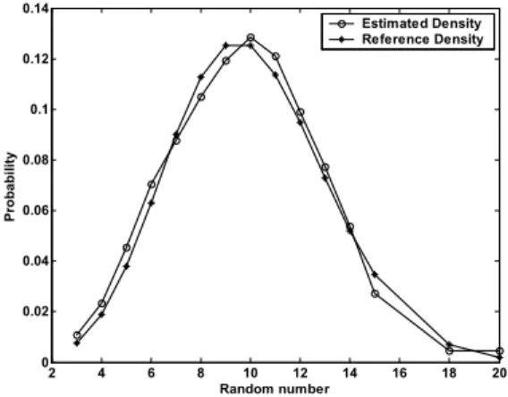
Fig. 5. Poisson random number (Example I). Initial values of α and β are randomly selected as uniformly distributed in [0,1] with the learning rate η = 0.5. Recursive learning continues until a specified error tolerance is reached. The error function is the average absolute difference between a reference probability p*

and the estimated probability P i.e.

∑ ∑ ∑

∑

= = = =                 − = = T n N i i N j j j n ij T n n z P z x x P J 1 1 1 , 1 , ) ( ) , ( ln max )} ( ln{ max β φ α β α β α (24)

Training is accomplished as in Example I. For comparison, the histogram method is additionally performed using the MATLAB command hist. The simulation results are given in Fig. 9. The results appear acceptable in comparison with those of the histogram approach.

∑

= − = N n x P x P N e 1 *_{( ) ( )} 1 (29) In the training simulation, 100 training data samples at each time k were temporally generated. Fig. 6 illustrates simulation result of the estimated probabilities along with the reference values. The plot shows that the estimation errors are less than 0.01 at all data point with an average error value of 0.0089.

0 20 40 60 80 100 120 140 0 0.01 0.02 0.03 0.04 0.05 0.06 0.07 Random number Pr o b a b ility Estimated Density Histogram 2 4 6 8 10 12 14 16 18 20 0 0.02 0.04 0.06 0.08 0.1 0.12 0.14 Random number Pr o b a b ility Estimated Density Reference Density

Fig. 9. Estimated probability (Example II). 6. DISCUSSION

Fig. 6. Estimated probability (Example I).

We propose a probability estimation approach using DBN. The method was successfully used to estimate discrete non-Gaussian signals. From the simulation results, we conclude that the performance of the approach is acceptable.

Example II: We nonlinearly transform Poisson random

data in this Example. To simulate this scenario, a random input is fed to a nonlinear system and the probabilities of the system output are estimated. A block

diagram for this process is depicted in Fig. 7. In future work, we will address the estimation of more complex distributions such as multi-variable non-Gaussian or non-stationary stochastic models. To this end, we will utilize and compare well-known algorithms such as the Viterbi algorithm [13].

Nonlinear system

x y _EstimatorDensity P(y)

Fig. 7. Transformation of a random variable.

ACKOWLEDGEMENTS The random input is Poisson distributed with the same

parameters as Example I. Because the data is nonlinearly transformed, the output probabilities are not Poisson and the output distribution is of an unknown form. We define the nonlinear function as y = cx3_(k)

where c is constant and generate 500 random input values. A time history of the output is shown in Fig. 8.

The authors are grateful for the support of NRL, National Research Laboratory in Dong-A University, Korea.

REFERENCES

[1] Richard O. Duda, Peter E. Hart, and David G. Stork, Pattern classification, A Wiley-Interscience Publication, NY, 2001. 0 100 200 300 400 500 0 20 40 60 80 100 120 140 Sample number R a nd om n u m b er

[2] E. Parzen, “On estimation of a probability density function and mode,” Analysis of Mathematical

statistics, Vol. 33, pp. 1065 - 1076.

[3] S. Fiori and P. Bucciarelli, “Probability density estimation using adaptive activation function neurons,” Neural Processing Letters, Vol. 12, pp. 31-42, 2001.

[4] M. Strikanth, H. K. Kesavan, and P. H. Roe, “Probability density function estimation using the MinMax measure,” IEEE Trans. on Systems, Man,

and Cybernetics-Part C: Applications and Reviews,

Vol. 30, No. 1, pp. 77-83, 2000. Fig. 8. Poisson random number (Example II).

[5] A. Sarajedini, R. Hecht-Nielsen, and P. M. Chau, “Conditional probability density function estimation with sigmoidal neural networks,” IEEE

Trans. on Neural Networks, Vol. 10, No. 2, pp.

231-238, 1999.

[6] G. Miller and D. Horn, “Maximum entropy approach to probability density estimation,”

International Conference on Knowledge-Based Intelligent Electronic Systems, Vol. 1, pp. 225-230,

1998.

[7] K. Sharifi and A. Leon-Garcia, “Estimation of shape parameter for generalized Gaussian distributions in subband decompositions of video,”

IEEE Trans. on Circuits and Systems for Video Technology, Vol. 5, No. 1, pp. 52-56,1995.

[8] D. S. Modha and Y. Fainman, “A learning law for density estimation,” IEEE Trans. on Neural

Networks, Vol. 5, No. 3, pp. 519-523, 1994. [9] Y. Baram and Z. Roth, “Forecasting by density

shaping using neural networks,” IEEE/IAFE Proc.

of Computational Intelligence for Financial Engineering, pp. 57-71, 1995.

[10] J. M. Mendel, Lessons in estimation theory for

signal processing, communications, and control,

Prentice Hall, NJ, 1995.

[11] F. V. Jensen, Bayesian networks and decision

graphs, Springer, NY, 2001.

[12] D. Heckerman, “A tutorial on learning with Bayesian networks,” Technical report

MSR-TR-95-06, Microsoft Research, Washington,

1996.

[13] G. D. Forney, “The Viterbi algorithm,” Proc. of