This study comprehensively investigates the wage structure determinants and gender pay gap in Korea. Using 2014 Korean Labor and Income Panel Study (KLIPS) data, we find that individual characteristics exhibit significant differences across the distribution and that magnitude and significance differ according to gender.
Findings suggest that returns to education are high for women and experience is influential only for women at the upper wage distribution. By applying vigorous counterfactual decomposition method, we find large returns on characteristic differentials by gender, especially for lowly educated women. A strong glass ceiling effect in Korea is obtained, and the integrative effect is composed of the continuously increasing composition effect and N-shaped (i.e., low at both ends) structure effect. In particular, most of the explained differentials are attributable to the differences of experience. The high returns on education for women are beneficial for reducing discrimination (unexplained or structure effect).
Keywords: Glass ceiling effect, Korean gender pay gap, Uncondi- tional quantile regression
JEL Classification: J31, J71
HongYe Sun, Department of Economics, Pusan National University, 30 jangjeon-dong, geumjeong-gu, Pusan, South Korea. (E-mail): hysun@pusan.
ac.kr; GiSeung Kim, Corresponding author, Department of Economics, Pusan National University, South Korea. (E-mail): [email protected], (Tel): 051-510- 2564, (Fax): 051-581-3143, respectively.
This work was supported by a 2-year Research Grant of Pusan National University.
[Seoul Journal of Economics 2017, Vol. 30, No. 1]
Gender Pay Gap among Wage Earners:
from Mean to Overall Log Wage Distributional Decomposition
HongYe Sun and GiSeung Kim
I. Introduction
Considerable research on gender pay inequality shows that gender pay inequality is relatively higher in Korea than in other industrialized countries. As citizens of a developed and high-income OECD member country, women in Korea face more severe employment stresses than women in similar countries. The average gender wage gap for OECD countries decreased from 23.1 in 2000 to 17.5 in 2014.1 However, the gender wage differentials in Korea topped this list in 2000 (41.7) and did not decrease to the same extent by 2014 (36.7, remained the first) as in other advanced OECD countries. With respect to other labor market characteristics, the labor force participant rate of 74% and 47% for men and women in 2000 changed to 74% and 49.2% in 2014. This change trend is comparable to the change from 73.7% and 50% for men and women in 2000 to 69.2% and 55.4% in 2014 for the OECD average.
For educational attainment, the average educational level for Koreans significantly exceeds the OECD average, with 48% of men and 41% of women attaining tertiary degrees in 2014. Around 73.9% of the total working population in the country was working in 2015.
A large gender pay gap in Korea is well documented using various analytical frames and control variables. The present study investigates the gender pay gap for Korean wage earners. Gender pay gap is attributable mainly to observable productivity differential and unobservable discrimination. According to Becker (1971), discrimination unrelated to an individual’s productivity is harmful to workforce optimization and social productive efficiency. Korea’s significantly wide gender earnings gap is attributed to the stiff job market for women and poor social services for working mothers.2 Korea women typically have to quit their jobs when they give birth3, and their rate of return to full-
1 For full-time employees, the gender wage gap is unadjusted and defined as the difference between male and female median wages divided by the male median wages.
2 Becker (1985) suggested that the less productivity for women than men with similar human capital characteristics may be related to energy decentralizing because of housework and childcare leave.
3 Although the average fertility rate in Korea is 1.21 (as compared to the OECD average of 1.68 in 2014), the pressure of child care is relatively high for Korean mothers.
time work is low.4
Considering the large gender pay gap in Korea, we precisely investigate the gender imparity. The classical human capital theory explores the productivity difference by gender on wage structure. The dominant human capital components in wage structure are education, experience, and job training. Educational attainment significantly influences individuals’ incomes in Korea and other countries. However, given the high average educational level, the returns to education may be lower in Korea than in other countries. Meanwhile, the importance of experience may obviously increase in magnitude.
The unobservable ability related to education in the error term may result in incorrect regression returns to education, that is, the endogenous estimation bias. To overcome the endogenous problem, economists proposed three major solutions for eliminating the variable bias. These solutions are using a proxy variable, using a twin sample in terms of fixed effect model, and using an instrumental variable. We adopt the proxy variable method to solve the ability bias problem in this study because of the sample and variable limitation. The common proxy variables are intelligence quotient (IQ), work assessment score, and family background. Following earlier literature, we adopt father’s education as the proxy of ability. In general, ability is categorized into cognitive ability and non-cognitive ability. Estimating human capital factors of wage structure without considering the effect of non-cognitive ability may cause serious estimation bias (Heckman, and Rubinstein 2001). In addition, non-cognitive abilities significantly influence pooled sample earnings structure and lead to different estimated results by gender.5 Therefore, we adopt life confidence as a non-cognitive ability proxy that reflects individual’s endeavor motivation.
Most earlier studies on gender pay differentials focused only on the analysis at the mean of the distribution. However, failing to consider the pay gap across the overall distribution may hinder the thorough
4 Arulampalam et al. (2007) determined two possibilities about the relationship between working women and childrearing women. One is that pay compression results in leaving work force, and the other is that high wage floors lead to high work force stay likelihood. They noted that the pattern variation of gender pay gap across the wage distribution needs to be empirically studied.
5 Personal characteristics affect the decrease of gender pay gap and overall wage inequality (Antonczyk et al. 2010).
investigation of the comprehensive reality. Since Koenker, and Bassett (1978) proposed the quantile regression (QR) method, the limitation on mean regression has been resolved and estimation has been expanded across the overall distribution. Research on wage structure and gender pay gap has spread to the overall wage distribution for the Korean labor market, but published findings remain scarce. The two major drawbacks of previous studies are summarized as follows. First, for the traditional QR method, the estimated coefficient cannot reflect the real effect of the explanatory variable on the explained variable. Indeed, the QR estimation results of Koenker, and Basset (1978) present the effect of the explanatory variable on the conditional distribution. Therefore, the typical QR method is also called conditional QR (CQR). Second, for the decomposition of gender wage gap, the popular Oaxaca–Blinder (1973) technique and other conditional decomposition methodologies are suitable only to the decomposition of mean earnings differences in terms of linear regression models. These models mask further gender pay decomposition across the overall earnings distribution.
To solve these limitations of previous studies, we apply unconditional QR (UQR) and counterfactual distribution decomposition by Firpo et al. (2009) to further exploit the mechanism of wage structure and decompose the gender wage gap beyond the mean distribution. Firpo et al. used UQR to show the direct marginal effects of the explanatory variable on the specific unconditional quantiles intuitively, basing on the re-centered influence function (RIF) that reflects the real interest in economic applications. Furthermore, we adopt the counterfactual distribution decomposition method (Machado, and Mata 2005;
Melly 2006; Autor et al. 2006) to decompose the gender wage gap across overall distributions. Machado, and Mata (2005) proposed the original decomposition method based on CQR and constructed the counterfactual distribution through the estimation of marginal density function in terms of probability integral transformation. Their alternative decomposition procedure (MM-2005 hereinafter) combines QR and bootstrap approach to estimate counterfactual density functions. MM-2005 provides a valid way to decompose gender wage gap into the composition effect (endowment) and the structure effect (discrimination) across the distributions. However, with a large dataset, the MM-2005 method is computationally demanding (time consuming) and does not offer the sub-component decomposition approach. Melly (2006) and Autor et al. (2006) further developed the counterfactual
distribution decomposition method. Their refined method revised the cross-line problem among different quantiles and improved the estimation efficiency. However, Melly (2006) and Autor et al. (2006) did not overcome the drawbacks of MM-2005, and the decomposition component (composition and structure effects) is subject to the selection of the individual’s characteristic variable with self-determination. To overcome this limitation of MM-2005 and the decomposition of Melly (2006) and Autor et al. (2006), we adopt RIF in conjunction with the Oaxaca–Blinder method (RIF-OB) based on UQR to further exploit the composition and structure effects on each explanatory variable. These explorations can help obtain knowledge on the extent of the gender pay gap in Korea, the main component that causes such gender pay gap, and whether this gender wage gap varies across the overall pay distribution.
The rest of the paper is organized as follows. Section II reviews the previous literature. Section III discusses the analysis data and describes the summary statistics of men and women. Section IV outlines the research models and explores the wage decomposition approach.
Section V presents the empirical results. Finally, Section VI summarizes the main conclusions and discusses policy implications.
II. Literature Review
Literature on gender wage gap is abundant and focused mostly on decomposing the earnings gap on the mean wage distribution. However, as noted in many previous studies, the characteristic heterogeneity of men and women across the overall distribution may significantly affect the pattern of gender wage gap. Later studies confirmed the evidence of gender wage gap variance across the distribution. The extension of the decomposition methodology provided highly efficient estimation of the gender wage differentials.
With respect to the profile of gender pay gap across the overall wage distribution, Albrecht et al. (2003) originally adopted QR and verified the glass ceiling effect hypothesis in Sweden. They found that the largest gender pay gap and discrimination exist against women at the top tail of the wage distribution. After this study, various studies exploring the gender wage gap across the distribution covered most of the developed and developing countries.
To date, the findings indicate that the glass ceiling effect6 is found mainly in developed countries and that the sticky floor effect7 (i.e., large gender wage gap or discrimination at the bottom of the distribution) generally exists in developing countries (Carrillo et al.
2014; Chi, and Li 2008). The glass ceiling effect has been confirmed in most developed Western countries (e.g., Jellal et al. 2008 for France;
Matano, and Naticchioni 2013 for Italy; Russo, and Hassink 2012 for the Netherlands). Several early studies covered multiple European countries (Arulampalam et al. 2007; Christofides et al. 2013; Perugini, and Selezneva 2015). Using the sample of European Union Statistics on Income and Living Conditions in 2007 and 2009, Perugini, and Selezneva (2015) investigated the adjusted gender wage gap across the overall distribution in 10 Eastern Europe countries. They also suggested that seven countries face significant glass ceiling effect, except Romania, Slovenia, and the Slovak Republic. Using a large-scale survey from the European Community Household Panel, Arulampalam et al. (2007) found a glass ceiling effect in most European countries.
Using EU Statistics on Income and Living Conditions 2007 data, Christofides et al. (2013) examined the gender wage gap in 26 European countries and discovered a large gender pay gap at the upper tail of the wage distribution in a number of relatively advanced countries. They also observed the existence of the sticky floor effect in 11 European countries, but found no evidence of effect in either Latvia or Lithuania.
Baert et al. (2016) indicated that women encounter stronger resistance than men in climbing the career ladder. In Britain, the glass ceiling effect is exhibited as full-time working women predominantly suffering from discrimination when they have the same characteristics, in particular for the high skilled, high-end occupations (Chzhen, and Mumford 2011).
Improving women’s educational attainment is acknowledged as a feasible pathway in narrowing gender pay gap. Over time, raw wage differentials worldwide have fallen substantially mostly because of good
6 The glass ceiling effect concept implies that the work of highly educated women is devalued or their promotion opportunities are limited (Arulampalam et al. 2007).
7 Booth et al. (2003) first defined a sticky floor as wage situation arising for women and tending to the same pay scale with men, and obtained that the gender differences of pay scale are large at the bottom wage distribution.
labor market endowments of females (Weichselbaumer, and Winter- Ebmer 2005). Nevertheless, some studies showed large gender earnings differentials in highly educated groups in some countries (Bobbitt-zeher 2007). Using survey data for Spain in 1995 and 1999, De La Rica et al. (2008) and del Río et al. (2011) found that highly educated women suffer considerable discrimination at the upper distribution, that is, the glass ceiling effect. They also reported that lowly educated women suffer from the sticky floor effect. The gender wage gap pattern over the distribution may vary according to specific research groups and objectives. Albrecht et al. (2009) explored and clarified the evidence of the glass ceiling effect among full-time workers in the Netherlands by applying the QR decomposition technique by Machado, and Mata (2005).
Kee (2006) found a glass ceiling effect in the private sector by applying the counterfactual decomposition, but found no evidence of either the sticky floor effect or the glass ceiling effect in the Australian public sector. Miller (2009) conducted a similar study in the United States and found results inconsistent with those of Kee (2006). They revealed the sticky floor effect in the public sector, but found neither the glass ceiling effect nor the sticky floor effect in the private sector. Mussida, and Picchio (2014) examined the glass ceiling effect in Italy and concluded that the effect is strong for highly educated women, while discrimination presents a steep increasing trend from lower to upper wage distribution toward women. Furthermore, Carrillo et al. (2014) investigated 12 Latin America countries and found that most countries are stuck in the sticky floor even when the wage differences are already partially masked by women’s higher educational attainment than men.
Given that the level of economic development and cultural background may clearly affect gender imparity, the gender wage gap situation across Asian countries with characteristics similar to those of Korea must be investigated. Using MM-2005, Ge et al. (2011) found the glass ceiling and sticky floor effects in Hong Kong. They attributed the majority of the gender pay gap at the upper distribution to differences in rewards to the productivity characteristics of men and women. The economic development level varies among Asian countries. Industrialized countries, such as Korea, Japan, and Singapore, have many highly educated workers, but most other Asian countries experience advanced labor scarcity. Using six Latin American countries and six Asian countries data from various sources, Fang, and Sakellariou (2015) suggested that the glass ceiling effect is prevalent in
most Latin American countries, while the sticky floor effect is frequent in Asian countries. They also indicated that the glass ceiling effect prevails in the public sector but varies significantly across the private sector of each country. Ahmed, and McGillivray (2015) examined the gender wage gap in Bangladesh from 1999 to 2009 using the extent of decomposition ranging from mean (the Oaxaca–Blinder method) to overall distribution (the Counterfactual and Wellington method). They found the sticky floor effect in Bangladesh and suggested that the gender wage gap narrows during the analysis period. The significant contractive trend of pay gap results mainly from the increasing women’s educational attainment and declining women’s discrimination. Chi, and Li (2008) and Xiu, and Gunderson (2014) found the sticky floor effect in China by applying urban household survey data of 1987, 1996, and 2004, and the Life Histories and Social Change in Contemporary survey in 1996. Chi, and Li (2008) attributed the phenomenon to the bottom of the distribution with low human capital endowment, whereas Xiu, and Gunderson (2014) suggested that coefficient differences (caused by discrimination) account for the large pay gap. With respect to other studies on Asia countries, Fang, and Sakellariou (2011), Gunewardena et al. (2008), Sakellariou (2004), and Sakellariou (2006) applied several different counterfactual decomposition methods over the distribution and found consistently clear evidence of the sticky floor effect in Thailand, Philippines, Singapore, and Sri Lanka.
After the commencement of Korea’s rapid economic growth in the 1960s, studies focusing on Korean gender pay inequality began to appear in the 1990s. These studies revealed that female wages in Korea increase more rapidly than those of men from the 1980s to 1990s (Berger et al. 1997). The literature also suggested that the gender wage gap narrows mainly because of the increase in women’s productivity characteristics, whereas the discrimination does not improve throughout the period (Berger et al. 1997; Turner, and Monk- turner 2006; Yoo 2003). Turner, and Monk-turner (2006) used the Occupational Wage Bargaining Survey on the Actual Condition and explored the change of the gender wage gap in 1988 and 1998. By applying the Oaxaca (1973) decomposition, they found that the wage differentials decrease in magnitude although the gender wage gap exists at a high level throughout the decade. Furthermore, some studies explored the differences in gender inequality between Korea and other advanced countries. Contrary to the gender wage gap in the
United States, that in Korea is larger; experience, current job tenure, and educational attainment play a dominant role in explaining the differentials (Cho 2007). Using data from 2005 Korean Labor and Income Panel Study (KLIPS) and Panel Study of Income Dynamics (PSID), Cho et al. (2010) further compared the gender wage gap in Korea and the United States with respect to the private and public sectors.
They found that the gender wage gap is relatively higher in the Korean labor market than in other countries and suggested that discrimination accounts for the major share of total wage differentials. Furthermore, they attributed the relatively low wage gap in the Korean public sector to the pattern of women with high human capital entering the public sector. However, these studies have insufficiently investigated the overall wage distribution. Cho et al. (2014) exploited the gender wage gap under a stratified labor market view in terms of the counterfactual decomposition presented by Chernozhukov et al. (2009). Considering the dual labor market characteristic in Korea, they divided the labor market into the core sector (superior working condition) and the peripheral sector (inferior working condition). Their findings implied that women encounters strong and weak glass ceiling effects in the peripheral and core sectors. Moreover, discrimination is relatively higher toward women in the peripheral sector than women in the core sector.
III. Data and Summary Statistics
This study uses KLIPS dataset surveyed in 2014. The Korea Labor Institute began to collect detailed data of households and individuals in 1998. The essential survey objective of KLIPS includes personal income, social population characteristics, health, mobility, social lifestyle, social attitude, labor market, and social security. This data collection is modeled after processing, which is similar to the PSID from the University of Michigan. Among the individual observations, those who are currently employed as wage earners and have stated an average monthly income are selected. Thus, those who are currently self-employed or unemployed are excluded. Finally, our sample size is adjusted to 2,576 individual observations. Missing values for any of the explanatory variables that must be covered in our analysis are also excluded.
Table 1 presents the summary statistics with respect to the individual’s basic information, wage, experience, and education.
Considering the labor market characteristics in Korea, we set the age range from 18 years to 65 years. Men’s average age is 2 years older than women’s average age. Men are slightly more highly educated than women.8 Experience9 shows a gender gap consistent with previous studies: because of baby-caring and maternal responsibilities, Korean women must interrupt their work and experience difficulty in returning to work. This scenario reduces the women’s level of experience. After the data are trimmed, the final sample contains 1,538 men and 1,038 women wage earners. This result reflects that the men’s labor force participation rate is approximately 50% higher than that of women.
KLIPS contains the survey of monthly earnings and weekly working time of wage earners. Therefore, we calculate the hourly wage by
8 The judgement relies on the average education attainment and standard deviation for men and women. Year of education is calculated by the highest degree (8 categories: 0, 6, 9, 12, 14, 16, 18, and 22 years).
9 Experience is calculated by the survey year (2014) minus the individual’s latest job start year.
Table 1
Summary StatiSticSby gender
Men Women Norm.
Diff.
Mean S.D. Min Max Mean S.D. Min Max Hourly wage 1.66 0.82 0.35 4.46 1.02 0.51 0.32 4.46 0.55 Log Hourly Wage 0.39 0.49 −1.06 1.50 −0.08 0.43 −1.15 1.50 0.58
Age 42.47 10.15 19 65 40.10 10.99 18 65 0.16
Education 13.89 2.64 6 22 13.18 2.71 0 22 0.19
Experience 7.95 7.72 0 40 4.93 5.27 0 37 0.31
Experience2/100 1.23 2.14 0 16 0.52 1.15 0 13 0.28 Father’s
education 8.76 4.47 0 20 8.77 4.41 0 20 0.00
Number of
Observations 1,538 1,038
Note: The currency unit is 10,000 KRW.
Norm.Diff. denotes normalized difference calculated by the formula λδ = δ1 – δ0 /
λδ δ= 1−δ0/ σ12+σ02, where δ1 and δ0 means the sample mean, and σ12 and σ02 are the sample variances of men and women.
applying the formula of monthly wage /4.3*weekly working time.10 The average hourly wage is 16,600 and 10,200 KRW for men and women, respectively.
Table 2 shows the detailed information of the labor market characteristics by gender, including male and female wage and population share in terms of specific groups. As shown in Table 2, the dummy variables of individual characteristics include health, marital status, region, employment status, firm size, occupation, industry, and confidence. In our final selected analysis data, the distribution of dummy explanatory variables consists of the real labor market feature in Korea. The share of male regular employees is nearly 12% higher than that of female ones. Nearly 13% more men are married than women. For both genders, most respondents report having good health.
Furthermore, more respondents live in the capital area than in other areas. This relatively balanced distribution of region population helps us estimate an accurate result in view of the substantial economic gap between the capital and other areas. On the demand side of the labor market, firm size, occupation, and industry represent the essential characteristics. We divide firm size into three groups. We find that more than half of women are employed by small firms (< 30 employees), whereas most men are employed by large firms (> 300 employees). We categorize the 4-digit occupation from the raw data into five based on the International Standard Classification of Occupation. Furthermore, industry is categorized into five, from agriculture to government service.
Occupation and industry segregation by gender has been widely clarified by various studies with respect to the Korean labor market.
Unsurprisingly, we find the polarization phenomenon of occupation and industry between men and women. More women are gathered as office workers (clerical) than men. However, the distribution of occupation for men is relatively equal; except the bottom low-end occupation, the observations’ share of each occupation is around 20%. The finding of the relatively high wage in high-end occupations may be related to high-earning occupation, which requires workers (i.e., women) to accept more years of schooling. In addition, we find substantial occupation and industry segregation, and the results reveal a large earnings gap by gender in terms of descriptive statistics.
10 We trim the extreme value of hourly wage.
Table 2
compariSonof Labor market characteriSticSbetween menand women
(1) (2) (3) (4) Mean
value T – Stat.
Men Women Men Women Men Women W/M (%)
Seoul capital area 48.7 51.5 1.70 1.08 121.5 77.7 63.5 14.81***
Other areas 51.3 48.5 1.61 0.96 114.9 68.7 59.6 16.64***
Regular employment
81.5 69.8 1.77 1.13 126.9 80.8 63.8 18.68***
Non-regular
employment 18.5 30.3 1.12 0.77 79.8 55.1 68.8 10.18***
good health 76.9 62.8 1.79 1.05 128.1 75.0 58.7 20.17***
Below good health 23.1 37.2 1.19 0.97 85.1 69.6 81.5 6.17***
Married 70.0 61.6 1.72 1.07 123.1 76.6 62.2 17.71***
Unmarried 30.0 38.4 1.49 0.94 106.7 67.2 63.1 12.40***
Union members 23.2 13.3 2.24 1.48 160.3 105.8 66.1 8.91***
Non-union members
76.8 86.7 1.48 0.95 105.4 67.9 64.2 19.61***
Strong confidence 56.5 56.7 1.79 1.09 127.9 78.1 60.9 17.15***
Weak or lack confidence
43.5 43.3 1.48 0.93 105.5 66.3 62.8 14.59***
Firm of <30
employees 40.6 56.6 1.25 0.87 89.2 61.8 69.6 14.07***
Firm of 30–300 employees
33.2 25.5 1.63 1.12 116.2 79.6 68.7 10.74***
Firm of >300
employees 26.2 17.8 2.32 1.38 165.6 98.8 59.5 12.48***
Occupation Management, professional, technical
23.1 28.6 2.00 1.20 142.8 85.8 60.0 13.67***
Clerical 21.5 27.5 1.95 1.22 139.4 87.5 62.6 12.61***
Service, skilled workers
19.1 16.4 1.46 0.73 104.1 52.3 50.0 13.42***
Sales, production 28.4 17.0 1.45 0.88 103.5 62.6 60.7 9.81***
Maintenance, manual workers
7.9 10.6 1.05 0.69 75.0 49.5 65.7 6.44***
IV. Methodology
A. Gender Wage Gap Decomposition of the Mean Distribution
The classical decomposition method by Oaxaca and Blinder was initially proposed in 1973 to explore gender wage gap. This method measures the magnitude of discrimination for the two specific groups in the labor market, thus helping in policy making and improving social efficiency. Thereafter, several studies applied this traditional strategy and spread the research to many countries. The Oaxaca–
Blinder method focuses on constructing a counterfactual earnings Table 2
(continued)
(1) (2) (3) (4) Mean
value T – Stat.
Men Women Men Women Men Women W/M (%) Industry
Manufacturing 36.3 21.2 1.75 0.95 125.2 68.1 54.3 14.11***
Construction, retail, wholesale, electrical
23.8 15.6 1.53 0.91 109.2 64.6 59.5 9.60***
Financial, insurance, real estate, facility
16.2 17.2 1.85 1.24 131.7 88.5 67.0 7.51***
Education, health, welfare, public
6.2 27.6 1.83 1.10 130.4 78.3 60.1 10.22***
Agriculture, food,
transport, repair 17.4 18.3 1.38 0.88 98.8 63.1 63.8 8.21***
Note: The currency unit is 10,000 KRW.
(1), (2), (3), and (4) denote the share of population, hourly wage, the ratio of specific group average wage over total’s, and the ratio of women’s specific group average wage over men’s, respectively.
“Seoul capital area” includes Seoul, Incheon, and Gyeonggi-do, and is also named as capital region by the Korean central government, or otherwise.
“Good health” denotes the self-reported health level smaller than 3, which is measured from 1 (very good health) to 5 (very bad health), or otherwise.
“Strong confidence” denotes the self-reported improvement possibility of social economic status level smaller than 3, which is measured from 1 (very strong) to 5(very weak), or otherwise.
structure and decomposing the mean differences in log wages based on linear regression models (Jann 2008). The results of Oaxaca–Blinder decomposition comprise two parts: one is attributed to the differences of characteristics, indicating that the wage gap can be explained by the endowment differentials of the two specific groups; and the other is attributed to the differences of returns to characteristics, indicating that the wage gap is unexplained or discrimination exists.
We assume two groups, namely, men (M) and women (F), in the labor market with equilibrium wages of WM and WF. The characteristic vectors containing human capital or labor market indicators are denoted as XM and XF. Based on the Mincerian wage equation, the estimation of the gender earnings model is described as follows:
= β µ+
lnW X (1)
where β is the regression coefficient vector or the wage structure.
Supposing the mean values of the characteristic vectors are X‾M and X‾F for males and females, respectively, then the difference of the mean wage can be formed as lnWM −lnWF =XMβM −XFβF. Furthermore, the equation can be transformed as follows:
* * *
lnWM −lnWF =(XM −XF)β +XM(βM −β )+XF(β −βF) (2) where β* is the non-discriminatory coefficient vector in the counterfactual structure. (XM −XF)β* represents the wage gap caused by the endowment differentials, and XM(βM −β*)+XF(β*−βF) reveals the discrimination. In solving this equation, the reference and treated groups must be specified. However, the selection of the reference group may produce a specified reference coefficient vector, which results in an estimation variable.
In the classical Oaxaca decomposition, if men are chosen as a reference vector, then discrimination exists toward women and none toward men. Thus, the model can be transformed as follows:
lnWM −lnWF =(XM −XF)βM +XF(βM −βF) (3) Given that the resulting variable depends on the reference vector, no completely reasonable judgment is made about the selection of the reference vector. Thus, further studies expanded the calculation on the
parameter vector. Reimers (1983) proposed a method to estimate the reference vector by applying a half-and-half weight on calculating the average coefficients over both groups. Therefore, the reference vector is
βR* =0.5βM +0.5 .βF
Thereafter, Cotton (1988) referred to a similar method that changes the weight to the sample share of the total wage earners. Cotton transformed the above-mentioned equation to βC* =(n NM )βM +(n NF ) .βF In this equation, N denotes the total sample size; nM and nF are the group sizes of men and women, respectively.
Neumark (1988) innovated the traditional strategy relying on the employer discrimination behavior model. Moreover, the method overcomes the upper and lower bound limitations of the estimators in Oaxaca, Reimers, and Cotton. Neumark indicated that reference vector can be calculated by pooled sample regression, such that wage structure is transformed into the following equation:
ln ln ( )( ( ) )
(( ) )( )
M F M F M F
M F M F
W W X X X I X
I X X X X
β β
β β
− = − + −
′ ′
+ − + − (4)
where X indicates a matrix of observed weight containing the male and female samples and I is the identity matrix. Furthermore, Oaxaca–
Ransom (1994) used ΩN to represent the fitted value of weighted matrix and expressed the weighted coefficient as βN* = ΩNβM +(I − ΩN)βF and
′ ′ − ′
Ω =N (X XM M +X XN N)1X XM M.
Although the matrix-weighted coefficient β*N is inclusive of the comprehensive characteristic information of the total sample and enables flexible estimation, the discrimination-underestimated problem persists because of the omitted variable bias (Fortin 2008; Jann 2008).
B. Expanding the Gender Wage Gap Decomposition across the Overall Wage Distribution
The Oaxaca–Blinder decomposition focuses on the conditional mean wage differentials. However, in the real labor market, gender wage differential poses a different pattern based on the different wage distributions. Hence, the glass ceiling effect (Albrecht et al. 2003) indicates that the wage differential is significant at the top of the wage distribution. In addition, the sticky floor effect indicates that the wage differentials are noteworthy at the bottom of the wage distribution.
Therefore, the exploration of the overall wage distribution can be regarded as a significant expansion of the previous results. Apart from the primitive quantile decomposition method by Juhn, Murphy, and Pierce (JMP) (1993), the MM-200511 technique employs the least absolute deviation method to estimate the Koenker et al. (1987) QR. Supposing that the number of the samples is n and the uniform distribution is τ, then Qτ(lnW|X) is implemented for n times regression to afford the counterfactual wage distribution {Xjβˆ}(j= ⋅ ⋅ ⋅1, , )n . The estimator is the linearly expected value of lnW conditionally on the distribution of X. βˆ is the vector of coefficients obtained from a set of characteristics combination.
The Melly (2006) decomposition suggests that the conditional quantile must be integrated over the range of covariates to estimate the counterfactual distribution (Thomschke 2015). Melly (2006) emphasized that the transfer of the probability integral cannot assure the estimation consistency in terms of the conditional distribution function or the total distribution function through the MM-2005 decomposition.
Furthermore, along with this concept, wage differential can be divided into the following factors:
τ(ln m−ln f) [(= βˆˆˆˆm f) (− βˆf f)]( ) [(τ + βˆm m) (− βˆm f)]( )τ
D W W X X X X (5)
where Dτ(lnWm−lnWf) is the raw wage differential between males and females at τ quantile. The first term on the right side of the function represents the characteristic differential, and the second term represents the coefficient differential.
To overcome the disadvantage of CQR, we further employ the RIF estimation approach. CQR is an extensive method of OLS regression, and this method provides estimation models for conditional mean functions and improved conditional quantile functions. However, the CQR retains some limitations for the estimation of a wage function by quantile distribution. Firpo et al. (2007) proposed an intuitive method to estimate QR based on RIF. RIF-OB regression can estimate the effect of covariance on the dependent variable directly and support the decomposition of detailed results on each explanatory variable. The
11 The MM-2005 decomposition is well suited to depict heterogeneous characteristic and coefficient effects across the overall wage distribution (Azam 2012).
implementation of RIF-OB decomposition is divided into two steps.
The first step reconstructs the wage distribution by DiNardo et al. (1996), reweighting function as composition effect and structure effect. The wage differentials between the two groups are attributed to the differences of characteristics or the return to characteristics. We assume that the wage distribution in the quantile is Qτ(F). Therefore, the wage distribution of men and women at τ percentile can be described as Qτ(Fm) and Qτ(Ff). Accordingly, the marginal distribution of counterfactual wage FC can be obtained, which means that the return to characteristics has no differential at the same earnings distribution for men and women. Thus, the wage distribution change can be obtained as follows:
( )m ( ) [ ( )f m ( C)] [ ( C f)]
Q Fτ −Q Fτ = Q Fτ −Q Fτ + Q Fτ −F (6) where the first and second terms on the right side represent the structure and composition effects, respectively. In the second step, each individual covariate must be calculated by a distribution statistics function through an influence function to analyze the distribution statistics. Thereafter, we transform RIF to obtain the statistical result of the consistent estimator about each variable through the influence function.
Finally, based on the expectation law, the RIF regression formula is obtained by rewriting the expectation of RIF as follows:
( ; , W) ( ( )) ( )
RIF W Q Fτ =Qτ + τ − ΨW Q≤ τ f Qτ (7) Where Ψ{ · } is the indicator function and f indicates the corresponding density function. The alternative variable can be estimated by OLS regression on a vector of covariates if RIF is linear. Firpo et al. (2009) provided another non-parameter estimation method to estimate the results if RIF is nonlinear. In particular, the gender wage differential at quantile τ can be decomposed as follows:
τ τ
τ(ln m−ln f)= m( ( )β τˆˆˆm −β τˆf( )) (+ m − f) ( )β τˆm +εm +εf
Q W W X X X (8)
where X‾ represents the vector of covariate averages; βˆm and βˆf are the counterfactual distributions that assume the returns to the labor market characteristics for men and women, respectively. X‾m(βˆm(τ) – βˆc(τ))
represents the structure effect on the τ quantile of the combination of each covariate for male and female laborers. (Xm−Xf) ( )β τˆm indicates the composition effect (endowment effect) on gender wage differential at the τ quantile of the combination of each covariate. ετm+ετf represents the approximation error term estimated by RIF regression method on the male and female wage functions.
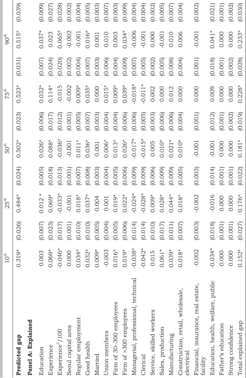
V. Empirical Results
A. Distributional Wage Determination on Quantile Wage Regression Conventional OLS estimation limit is used to depict the mean distribution of wage structure. In this section V, the findings reveal the returns to each explanatory variable and that the wage determinant mechanism varies across the distribution. Columns 5, 6, and 7 in Table 3 provide the results from the Firpo et al. (2009) UQR (resort to the RIF,12 also referred to as UQR) on the 10th, 50th, and 90th quantiles. For comparison, the result from Koenker and Bassett (1978) CQR13 is also reported in Table 3. The interpretation of coefficient in classical QR depends on the conditional distribution of covariates, and the result reflects the effect of explanatory variables on the conditional quantile.14 Contrary to the coefficient of CQR, the coefficient of UQR directly reflects the marginal effects of explanatory variables as OLS. Therefore, we only show CQR as a comparison to UQR estimation and do not provide further interpretation on the CQR results.15 In general, the wage determinant structure varies significantly across the distribution. The coefficient of returns to dominant factors changes in significance and
12 Influence function is a widely used tool in robust statistics (Firpo et al. 2009). The influence function represents the influence of an individual observation on a distributional measure of interest such as a quantile or other statistics (Magnani, and Zhu 2012).
13 The classical quantile regression is a parameter linear estimator and has the drawback of limited scope for interpretation. The explanatory variable regression coefficients in CQR are difficult to interpret and has low significant.
14 Unlike conditional means in a least squares regression, the average of conditional QR estimates does not coincide with the unconditional mean (Bosio 2014).
15 The detailed comparability analysis and application can be found in Firpo et al. (2009).
magnitude.
In particular, for the pooled sample, gender is clearly an important factor on wage across the distribution. However, the male premium on wage increases from the 10th percentile to the 50th percentile and peaks in the middle deciles. This finding also indicates that men receive a smaller gender premium at the top of the distribution than women.
Naturally, education significantly affects earnings across the full pay distribution. In light of the Mincer half elastic log wage model, the coefficient indicates that one additional year of education can bring approximately 1.6%, 3.5%, and 5.5% earnings increase at the 10th, 50th, and 90th percentiles, respectively. The returns to education increase from the 10th percentile to the 90th percentile, revealing that education significantly influences earnings at the top of the pay distribution.
The findings also correspond to the dual labor market, in which core sector employees receive high pay and returns to education, whereas peripheral sector employees suffer low pay and returns to education (Cho et al. 2014). Experience is another key human capital factor of wage structure. As discussed in Section IV, men have longer work experiences than women, and women’s work experience commonly emerges in a discontinuous pattern in the Korean labor market.
Notably, experience insignificantly affects wage at the upper percentile.
Apparently, the returns to experience increase from the 10th percentile to the 50th percentile and then decrease and disappear. Therefore, the coefficient of experience reveals that the factor of working years is important for the middle part of the distribution, but has a weak effect for the bottom and top parts of the distribution. The explanatory power of the determinant factor on wage structure is strong at the 50th percentile, indicating that many explanatory variables can be significantly estimated at the middle part of the distribution. Father’s education and confidence show opposite estimation significance. In particular, father’s education influences wages at the bottom of the pay distribution, whereas confidence significantly affects the wage structure for medium and upper pay distribution.
We find a strong firm size wage premium across the distribution, particularly for the top percentile. Contrary to employees in small firms (< 30 employees), employees in large firms (> 300 employees) gain a substantial earnings premium when they have the same characteristics.
The firm size premium on wage is large at the top of the pay distribution. Only a few of the explanatory variables show consistent
Table 3
wage Structure determinantSby QuantiLe regreSSion
CQR UQR
10th 50th 90th 10th 50th 90th
Constant -1.656***
(0.084)
-1.217***
(0.056)
-0.824***
(0.076)
-1.705***
(0.209)
-1.479***
(0.083)
-0.503***
(0.189)
Men 0.277***
(0.024) 0.318***
(0.019) 0.317***
(0.029) 0.270***
(0.050) 0.426***
(0.033) 0.188***
(0.040)
Education 0.033***
(0.006)
0.034***
(0.004)
0.034***
(0.005)
0.016**
(0.008)
0.035***
(0.005)
0.055***
(0.010) Experience 0.025***
(0.005)
0.027***
(0.004)
0.021***
(0.005)
0.009*
(0.005)
0.038***
(0.005)
0.006 (0.010) Experence2/100 -0.029
(0.021) -0.025*
(0.015) -0.012
(0.019) -0.026
(0.016) -0.087***
(0.015) 0.154***
(0.046) Seoul capital area 0.039
(0.026)
0.048***
(0.018)
0.031 (0.022)
0.035 (0.027)
0.050**
(0.022)
0.054 (0.033) Regular employment 0.133***
(0.043) 0.114***
(0.025) 0.113***
(0.034) 0.294***
(0.068) 0.109***
(0.032) -0.015 (0.026) good health 0.115***
(0.027)
0.119***
(0.017)
0.156***
(0.028)
0.020 (0.032)
0.153***
(0.025)
0.170***
(0.036)
Married 0.077***
(0.027) 0.023
(0.017) -0.012
(0.021) 0.072**
(0.033) 0.031
(0.025) 0.012 (0.037) Union members 0.090**
(0.036)
0.101***
(0.030)
0.084***
(0.028)
-0.020 (0.031)
0.098***
(0.031)
0.151**
(0.067) Firm of 30–300
employees 0.182***
(0.029) 0.144***
(0.017) 0.153***
(0.028) 0.157***
(0.030) 0.212***
(0.031) 0.075**
(0.034) Firm of >300
employees
0.292***
(0.038)
0.271***
(0.032)
0.278***
(0.039)
0.105***
(0.034)
0.294***
(0.033)
0.498***
(0.070) Manufacturing 0.123***
(0.036)
0.123***
(0.027)
0.096***
(0.032)
0.170***
(0.055)
0.133***
(0.033)
0.050 (0.055) Construction, retail,
wholesale, electrical 0.058
(0.042) 0.081***
(0.028) 0.091***
(0.035) 0.122***
(0.042) 0.097**
(0.039) 0.062 (0.045) Financial, insurance,
real estate, facility
0.105**
(0.042)
0.107***
(0.029)
0.109***
(0.037)
0.130**
(0.061)
0.139***
(0.040)
0.104*
(0.062) Education, health,
welfare, public 0.073
(0.049) 0.018
(0.033) -0.018
(0.039) 0.157**
(0.062) 0.036
(0.039) -0.116*
(0.066) Managerial,
professional, technical
0.275***
(0.067)
0.332***
(0.039)
0.332***
(0.049)
0.288***
(0.075)
0.375***
(0.050)
0.258***
(0.067)
significance and active direction on the wage structure across the distribution. Except firm size, health, union member, and education, most of the determinant variables present no influence on wage at the 90th percentile, implying that the wage premium only exists in the most essential or unobservable factors for the upper wage distribution.
The wage determinant mechanism presents a large difference for wage earners at different percentiles in Korea because of characteristic heterogeneity of individuals. Overall, the QR estimation results show the limitation of the mean estimation approach and emphasize the necessity of exploiting the wage structure across the full distribution.
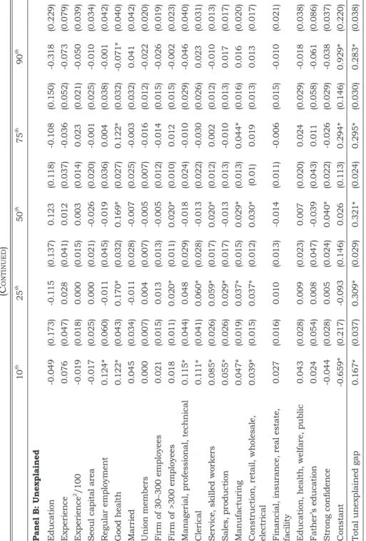
B. Unconditional Quantile Log Wage Regression for Men and Women In further exploring the wage determinant mechanism differences between men and women, Table 4 presents the results of RIF- unconditional regression estimates by gender at the 10th, 50th, and 90th percentiles. Early studies have widely verified the differences of wage structure for men and women. We find similar profiles of returns to education for men and women across the distribution and that
Table 3 (continued)
CQR UQR
10th 50th 90th 10th 50th 90th
Clerical 0.269***
(0.063)
0.240***
(0.034)
0.266***
(0.050)
0.321***
(0.071)
0.386***
(0.046)
-0.007 (0.073) Service, skilled
workers 0.164***
(0.054) 0.134***
(0.035) 0.182***
(0.051) 0.157*
(0.082) 0.235***
(0.043) 0.023 (0.046) Sales, production 0.080
(0.069) 0.080**
(0.033) 0.133***
(0.042) 0.210***
(0.072) 0.147***
(0.048) -0.082*
(0.047) Father’s education 0.003
(0.004)
-0.002 (0.002)
-0.001 (0.003)
0.007**
(0.003)
0.002 (0.003)
-0.005 (0.005) Strong confidence 0.041
(0.026) 0.059***
(0.015) 0.085***
(0.024) 0.041
(0.029) 0.058***
(0.022) 0.068*
(0.036) Pseudo R-squared 0.330 0.410 0.412 0.204 0.425 0.319
Observations 2,576 2,576 2,576 2,576 2,576 2,576
Note: *, **,* ** denote statistical significance at the level of 10%, 5%, and 1%.
Standard errors are in parentheses.
the regression coefficient for women is relatively higher than that for men. The findings are consistent with those of most studies on Asian countries (Chi, and Li 2008; Fang, and Sakellariou 2011). In addition, the fluctuation of returns to education for women is more considerable than that for men. Returns to education increase by 29% for men and 53% for women from the 50th to 90th deciles. The coefficient significance reflects the lack of any influence for education on earnings for men and women at the bottom of the pay distribution. On the contrary, education is the determinant factor of wage structure for the medium and upper pay distributions. A possible interpretation is the occupation segregation for lowly and highly educated groups. In other words, employees at the upper wage distribution with high-end occupation are prone to significantly benefit from enhanced educational attainment.
The pattern of experience is different for the two groups over the distribution. For men, long working experience improves earnings at the 10th and 50th percentiles, but no effect is found at the 90th percentile.
By contrast, for women, experience increases pay at the 50th and 90th percentiles but not at the bottom of the distribution. This finding may be related to male upper percentile wage earners being more apt to resort to high job skill or other talent instead of work experience.
Female bottom wage earners may be stuck in low-end occupations and at the risk of unemployment, and thus, they suffer nearly static wage increases with the growth of work experience. In general, only several individual and labor market characteristic variables (e.g., education, capital area, good health, confidence, and large firms) significantly affect the wage structure for the top of the pay distribution for men. Moreover, confidence has a significant influence on the wage at the upper percentile for men and women, indicating that non-cognitive ability has a similar effect regardless of gender for the upper distribution. In other words, employees at the upper wage distribution who have a positive attitude and confidence are likely to work hard and have a strong spirit of adventure. The findings reveal further that women working in large firms or engaged in managerial and professional occupation at the upper pay distribution can earn higher wages than the reference group.
In addition, the advantage in magnitude is significantly higher than that at the bottom of the pay distribution.
Considering the omitted variable bias, we adopt (Card 1995;
Ashenfelter, and Zimmerman 1997) the control variable approach16 and assume father’s education as a valid proxy variable. In omitting the ability bias problem, parental education is always an important issue on the role of ability proxy. No acknowledged and totally appreciated proxy variable is available for substituting unobservable ability. The most valid and commonly used variables are IQ, school score, and family background. Traditional OLS estimation has a downward bias estimation, and omitted ability variables induce an upward bias. If parental education is used as a valid proxy for an individual’s ability, then the inclusion of father’s education may reduce the upward ability bias. The resulting estimate also may be low.
We examine the regression coefficient with and without the ability proxy variable (father’s education and confidence), and find that the ability proxy variable induces 5% and 3% estimation decreases (mean distribution estimation) on returns to education for men and women, respectively.17 The instrument variable (IV) is also a common and feasible approach used to correct the omitted ability bias. The IV approach assumes that father’s education affects children’s educational achievements but is not correlated with children’s inherent abilities.18 Although the IV approach can correct the attenuation bias and the omitted variable bias, we do not adopt this method because of the limitation and effectiveness of the instrument.
C. Mean Wage Decomposition with Linear Regression
The Oaxaca–Blinder decomposition is a widely used method for exploring the gender wage gap across many countries. The decomposition technique is developed mainly to depict the pattern of gender wage throughout the full wage distributions. Showing the mean
16 The control variable approach is used to include proxy variables as additional regressors in the earnings equation to purge or absorb the effect of unobserved ability on the relationship between earnings and schooling. The underlying assumption is that parental education may sufficiently influence the extent of their children’s education and may thus be correlated to the capability or productivity of their children at work (Li, and Luo 2004).
17 Contact the authors for details.
18 The control variable approach assumes that parental education is correlated with an individual’s ability, but the IV approach assumes that they are not correlated.
Table 4
wage Structure determinantSacroSSthe DiStributionby gender
Men Women
10th 50th 90th 10th 50th 90th
Constant -1.797***
(0.199)
-1.021***
(0.101)
-0.152 (0.119)
-1.138***
(0.131)
-1.047***
(0.102)
-1.080***
(0.180)
Education 0.005
(0.010) 0.037***
(0.007) 0.052***
(0.009) 0.008
(0.008) 0.036***
(0.007) 0.076***
(0.013) Experience 0.023***
(0.008)
0.029***
(0.005)
0.007 (0.009)
0.007 (0.006)
0.027***
(0.006)
0.022*
(0.013) Experence2/100 -0.065***
(0.023)
-0.052***
(0.017)
0.092**
(0.038)
-0.029 (0.023)
-0.057***
(0.022)
0.189***
(0.067) Seoul capital area -0.001
(0.043) 0.035
(0.029) 0.082**
(0.033) 0.031
(0.025) 0.085***
(0.030) 0.102*
(0.052) Regular employment 0.292***
(0.080)
0.090**
(0.037)
-0.013 (0.035)
0.113***
(0.044)
0.117***
(0.038)
-0.011 (0.044) good health 0.226***
(0.062) 0.253***
(0.034) 0.115***
(0.029) 0.031
(0.032) -0.015
(0.032) 0.228***
(0.057)
Married 0.102*
(0.055)
0.012 (0.030)
0.007 (0.037)
0.029 (0.030)
0.023 (0.030)
-0.060 (0.057) Union members -0.030
(0.044) 0.063*
(0.035) 0.099
(0.079) -0.033
(0.023) 0.097***
(0.037) 0.267*
(0.139) Firm of 30–300
employees
0.210***
(0.055)
0.168***
(0.039)
0.035 (0.034)
0.126***
(0.032)
0.190***
(0.042)
0.137**
(0.068) Firm of >300
employees 0.233***
(0.061) 0.309***
(0.040) 0.411***
(0.069) 0.131***
(0.031) 0.195***
(0.041) 0.424***
(0.112) Manufacturing 0.259***
(0.064)
0.138***
(0.038)
0.065 (0.050)
0.037 (0.058)
-0.000 (0.043)
-0.011 (0.083) Construction, retail,
wholesale, electrical
0.225***
(0.074)
0.117***
(0.041)
0.076 (0.054)
-0.024 (0.062)
-0.076 (0.053)
-0.009 (0.100) Financial, insurance,
real estate, facility 0.153*
(0.085) 0.070*
(0.040) 0.090
(0.066) -0.002
(0.057) 0.153***
(0.046) 0.145 (0.096) Education, health,
welfare, public
0.158*
(0.084)
0.005 (0.059)
-0.193**
(0.095)
0.002 (0.056)
-0.021 (0.044)
-0.128 (0.102) Managerial,
professional, technical 0.692***
(0.125) 0.307***
(0.057) 0.113*
(0.058) 0.290***
(0.086) 0.370***
(0.067) 0.273**
(0.137)
Clerical 0.695***
(0.129)
0.248***
(0.057)
0.015 (0.059)
0.289***
(0.083)
0.297***
(0.062)
-0.068 (0.088)
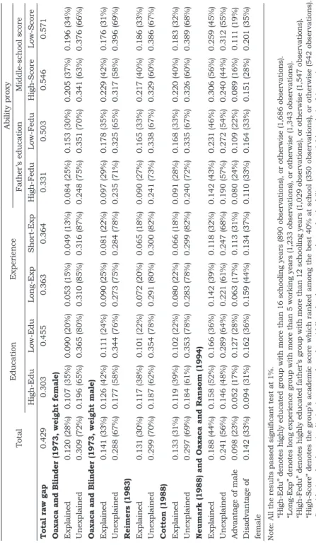
wage decomposition results and comparing subgroups horizontally in the Korean labor market are necessary. Table 5 presents the mean wage decomposition results by applying the Oaxaca (1973), Reimers (1983), Cotton (1988), and Neumark (1988) reference vector standard.19 Considering that the differences in human capital background may considerably affect the wage gap, we divide the total sample further into several subsets to investigate the mean wage gap profiles. As discussed in Section III, the results of Reimers (1983) and Cotton (1988) confirm that the coefficient is always stuck between the upper and lower bounds (i.e., Oaxaca female and male weights). For the total sample, the decomposition results do not show considerable difference among the methods of Oaxaca (1973), Reimers (1983), and Cotton (1988); the share of explained (endowment) gap is around 30%, whereas the unexplained (discrimination) gap is around 70%. The Neumark (1988) and Oaxaca–
Ransom (1994) methods break the bound limitation and reveal the ratio of explained and unexplained variables as 44% and 56%, respectively.
The results of the standard Oaxaca decomposition indicate that
19 Neumark (1988) and Oaxaca, and Ransom (1994) adopt a similar method to construct the no-discrimination wage structure.
Table 4 (continued)
Men Women
10th 50th 90th 10th 50th 90th Service, skilled
workers
0.566***
(0.131)
0.193***
(0.048)
-0.010 (0.047)
0.048 (0.085)
0.070 (0.050)
0.051 (0.068) Sales, production 0.531***
(0.127) 0.085*
(0.047) -0.006
(0.038) 0.207**
(0.091) 0.162***
(0.054) -0.107 (0.097) Father’s education 0.004
(0.006)
-0.002 (0.003)
-0.002 (0.005)
0.001 (0.003)
0.003 (0.004)
0.005 (0.009) Strong confidence -0.012
(0.039) 0.096***
(0.026) 0.084**
(0.036) 0.065**
(0.029) 0.026
(0.028) 0.151***
(0.048) Pseudo R-squared
Observations
0.196 1,538
0.359 1,538
0.274 1,538
0.166 1,038
0.353 1,038
0.288 1,038 Note: *, **,* ** denote statistical significance at the level of 10%, 5% and 1%.
Standard errors are in parentheses.