Also, our device placement technique can leverage our performance model to avoid offline profiling. Our prediction model only takes less than a few seconds, while our device placement algorithm using the results from the modeling shows better training speed than the data parallelism as a basis. Our heterogeneous-aware hardware deployment achieves 1.12x for the VGG model compared to the baseline partitioning scheme, which does not consider heterogeneous GPU performance.
When heterogeneous groups of GPUs are used by different DNN jobs, different types of GPUs are used simultaneously to train a single network. The following questions are our motivating question for distributed training in heterogeneous GPU computing environments. However, since the efficiency depends on the model partition and the device placement of the partitioned model, the optimization of.
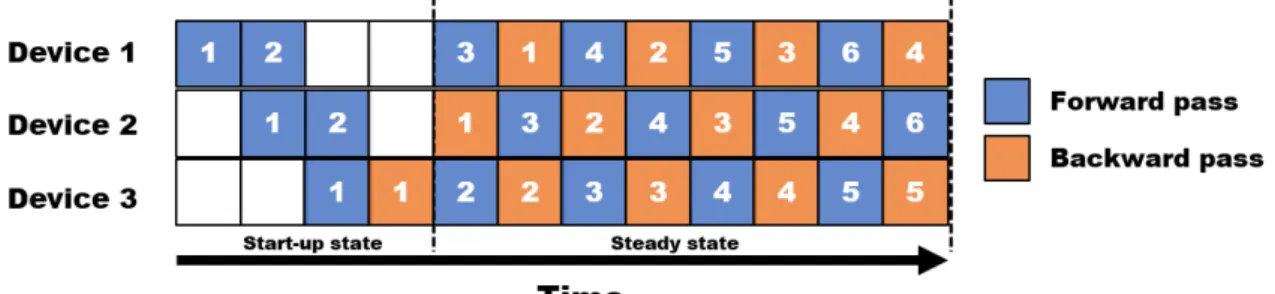
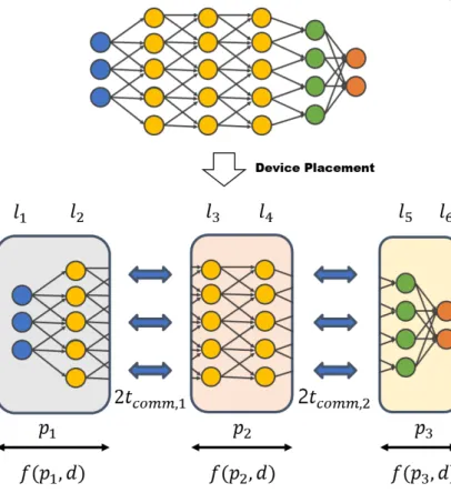
In order to be able to use heterogeneous GPEs to train a single DNN model, the heterogeneous performance of GPEs must be taken into account, which is a more complex problem. In this work, we discuss model partitioning and device placement to improve pipeline parallelism under heterogeneous GPE performance. For pipeline parallelism, it can have different computation and communication times depending on the device placement in the layer.
The performance model can help us avoid off-line profiling to obtain the necessary performance information for device placement algorithms or configurations for distributed executions.
Data parallelism
Model Parallelism
Pipeline Parallelism
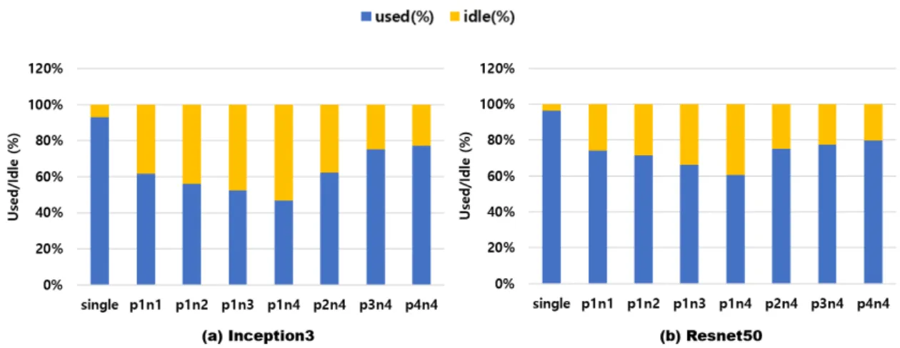
Straggler Problem
Motivation
Analysis
Because the parameter server and the worker server are on the same node, they will be w-1 instead of w. Model parallelism and pipeline parallelism Communication in model parallelism and pipeline parallelism occurs only between partitioned models. When the calculated activation output of one layer is transferred to the input of the next layer, it is transmitted over the network or PCI-E interconnect.
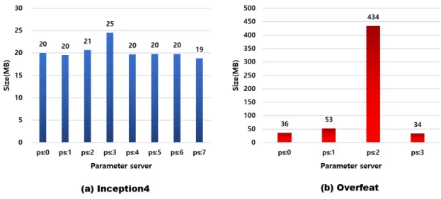
K is the array size and W, H and D are the width, height and depth of the activation output (the next layer's input data). In interlayer communication, since only one matrix is transmitted, a performance model for the communication time can be defined in a very simple form. When the training parameters are asymmetrically distributed on the parameter server, so the communication traffic applied to each parameter server is different.
For example, the distribution of parameters in inception3 is almost uniformly distributed due to similar size matrices, so similar load balancing is displayed for each parameter server. However, in the case of Overfeat, the size of some of the parameters is very large compared to others. Also, since parameter passing in the Tensorflow is performed by gRPC framework and multi-threading, mutually.
Therefore, the communication time modeling takes into account the load imbalance and the number of gRPC threads.

Methodology
This memory size is divided by the global memory bandwidth to obtain the memory read/write time. The final computation time is obtained by combining the core computation time and the memory read/write time. The formula below represents the method for calculating the computation time of an iteration time for a DL model.
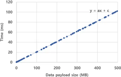
RW(l, d) represents memory read/write time reclaimed by all request bytes for input data, filter data and enable output data to read or write divided by memory bandwidth of device. Linear regression using synthetic data Figure 6 shows that synthetic data is generated and the actual transmission time is measured, and the linear relationship is shown as in the above analysis. The time required for one gRPC thread to transfer one matrix can be expressed by the following equation, and the coefficients are approximated by parameterizing them.
The only communication is between partitioned models, and the data transfer size is the same as the size of the activation output for the last layer of a partition. When multiple gRPCs transmit multiple parameters simultaneously, the number of gRPC threads, serialization/deserialization time, and interference between data transfers via shared resources such as network, PCI-E should be considered. Since serialization/deserialization uses the CPU core, it is assumed that it can be executed concurrently in a multi-core environment.
On the other hand, since transfer time uses network switch or PCI-E, gRPC threads interfered with each other. When multiple threads try to send its own parameter, 'Transfer' parts get a slowdown from each other while serialization and deserialization parts don't. The default value of the number of gRPC threads in Tensorflow is 8, so there can be at most 8 times latency.
We first analyze the architecture of a DL model and its parameter server and worker server configuration and discover one slowest worker and its parameters sent to or from a parameter server.
Result
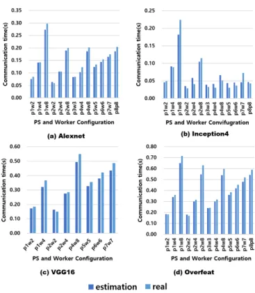
Each communication time was measured from the time parameter servers sent parameters to each work server until the time each worker finished receiving. Our communication model predicts these four models well and the overall average error rate is 13.79%. And we did not include small DL models in this result, because small DL models were not trained with distributed GPU execution.
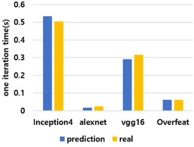
Total iteration time We combine computation prediction and communication prediction in iteration time. We see that this is because the computation time error rate for Alexnet was not negligible. Since Overfeat communication is dominant in a repetition time, Overfeat repetition time results appear to be similar to communication time.
Calculation time of the layer Figure 11 shows the comparison of the estimated calculation time and the actual calculation time. We run this experiment on the Overfeat model, VGG16 and Inception4 using two types of GPUs. The result shows an error in the prior layer and a relatively good predictor in the middle or posterior layer.
The reason that the front layers have a relatively large error is interpreted as the fact that the memory read/write cost is very high due to the large amount of input/activation output and filter size, so that the memory access time becomes a bottleneck. Since the per-layer error averages 25% over these three models and the front-layer error is large, better accuracy can be expected by improving the model memory read/write performance. This is because in pipeline parallelism, only one parameter array is sent by one gRPC thread, so no interference occurs.
Convolutional Network generally shows that the size of the data transferred from front to back is quite large, and shows that the performance modeling intuition is well suited.
Disccusion
Motivation
Methodology
To achieve the maximum efficiency of the pipeline, balancing the execution times of each step must be achieved. Since the execution time of the slowest step becomes the final iteration time for processing a minibatch in pipeline parallelism. This problem can be defined with a mini-max problem and can be formulated with an objective function and constraints.
We have formulated this optimization formula that can also be partitioned to use fewer GPUs than user-specified GPUs. This occurs when the communication time of any partition is dominant over the execution time of the partition.
System Overview
Result
The Hetero-Pipeline applies our device placement technique, and performance modeling is also applied considering communication times and performance of the heterogeneous GPUs. Equal- Pipeline, on the other hand, showed better speedup than data parallelism due to the effects of the pipeline, but no longer increases the efficiency of the pipeline through the skewed model partitioning. For the VGG16 model, the Hetero-Pipeline with the best model split was 1.42x and 1.12x faster than the data parallelism and equal-pipeline, respectively.
Because Overfeat has a small number of layers and each layer has a long computation time, splitting the model was very simple and shows the same device placement as Equal-Pipeline. For smaller and more layered models, the effect of the Hetero-Pipeline technique will be critical.
Discussion
Performance Modeling
Pipeline Parallelism
Agarwal, "Cntk: Microsoft's Open Source Deep Learning Toolkit," in Proceedings of 22nd International ACM SIGKDD on Knowledge Discovery and Data Mining, ser. Xing, "Addressing the Straggler problem for iterative convergent parallel ml," in Proceedings of Seventh ACM Symposium on Cloud Computing, ser. 9] “Efficient and robust parallel DNN training through model parallelism on multi-gpu platform”, CoRR, vol.
Guo, “Optimus: An efficient dynamic resource scheduling for deep learning clusters,” in Proceedings of the Thirteenth EuroSys Conference, ser. I would like to express my special thanks to my advisor Young-ri Choi for her patient guidance, enthusiastic encouragement and helpful criticism for this research work. I would like to express my appreciation to Professor MyeongJae Jeon who always listens carefully to my thoughts and words and motivates me to complete this research work.
Secondly, I would also like to express my appreciation to the following companies for their assistance and great help. Finally, I would like to thank my parents for their support and encouragement throughout my studies.