JHEP11(2016)024
Published for SISSA by Springer
Received: June 27, 2016 Revised: September 1, 2016 Accepted: October 16, 2016 Published: November 7, 2016
Massless and massive higher spins from anti-de Sitter space waveguide
Seungho Gwak,a Jaewon Kima and Soo-Jong Reya,b
aSchool of Physics and Astronomy & Center for Theoretical Physics, Seoul National University, Seoul 08826, Korea
bFields, Gravity & Strings, Center for Theoretical Physics of the Universe, Institute for Basic Sciences,
Daejeon 34047, Korea
E-mail: [email protected]
Abstract:Understanding Higgs mechanism for higher-spin gauge fields is an outstanding open problem. We investigate this problem in the context of Kaluza-Klein compactifica- tion. Starting from a free massless higher-spin field in (d+ 2)-dimensional anti-de Sitter space and compactifying over a finite angular wedge, we obtain an infinite tower of heavy, light and massless higher-spin fields in (d+ 1)-dimensional anti-de Sitter space. All mas- sive higher-spin fields are described gauge invariantly in terms of Stueckelberg fields. The spectrum depends on the boundary conditions imposed at both ends of the wedges. We ob- served that higher-derivative boundary condition is inevitable for spin greater than three.
For some higher-derivative boundary conditions, equivalently, spectrum-dependent bound- ary conditions, we get a non-unitary representation of partially-massless higher-spin fields of varying depth. We present intuitive picture which higher-derivative boundary conditions yield non-unitary system in terms of boundary action. We argue that isotropic Lifshitz in- terfaces inO(N) Heisenberg magnet orO(N) Gross-Neveu model provides the holographic dual conformal field theory and propose experimental test of (inverse) Higgs mechanism for massive and partially massless higher-spin fields.
Keywords: Higher Spin Gravity, Gauge-gravity correspondence, Higher Spin Symmetry ArXiv ePrint: 1605.06526
JHEP11(2016)024
Contents
1 Introduction 2
2 Flat space waveguide and boundary conditions 5
2.1 Kalauza-Klein mode expansion 6
2.2 Vector boundary condition 7
2.3 Scalar boundary condition 9
2.4 D3-branes ending on five-branes and S-duality 10
3 Waveguide in anti-de Sitter space 10
4 AdS waveguide spectrum of spin-one field 13
4.1 Mode functions of spin-one waveguide 13
4.2 Waveguide boundary conditions for spin-one field 19
5 Waveguide spectrum of spin-two field 21
5.1 Mode functions of spin-two waveguide 21
5.2 Waveguide boundary conditions for spin-two field 26
6 Waveguide spectrum of spin-three field 29
7 Higher-derivative boundary condition 33
7.1 Case 1: open string in harmonic potential 34
7.2 Spin-two waveguide with higher-derivative boundary conditions 39
8 Waveguide spectrum of spin-s field 44
8.1 Stueckelberg gauge transformations 44
8.2 Kaluza-Klein modes and ground modes 45
8.3 Waveguide boundary conditions 48
8.4 More on boundary conditions 49
8.5 Decompactification limit 51
9 Holographic dual: isotropic Lifshitz interface 52
10 Discussions and outlooks 53
A AdS space 56
B Verma module and partially massless(PM) field 56
C From (A)dSd+k to (A)dSd+1 57
JHEP11(2016)024
People used to think that when a thing changes, it must be in a state of change, and that when a thing moves, it is in a state of motion.
This is now known to be a mistake.
bertrand russell 1 Introduction
Massive particles of spin higher than two are not only a possibility — both theoretically as in string theory and experimentally as in hadronic resonances (See, for example, [1])
— but also a necessity for consistent dynamics of lower spin gauge fields they interact to (See, for example, [2]). As for their lower spin counterpart, one expects that their masses were generated by a sort of Higgs mechanism, combining higher-spin Goldstone fields [3,4]
to massless higher spin gauge fields. Conversely, one expects that, in the massless limit, massive higher-spin fields undergo inverse Higgs mechanism and split its polarization states irreducibly into massless higher-spin gauge fields and higher-spin Goldstone fields. On the other hand, it is well-known that the higher-spin gauge invariance is consistent only in curved background such as (anti)-de Sitter space ((A)dS). As such, gauge invariant description of massive higher-spin fields and their Higgs mechanism would necessitate any dynamical description of the (inverse) Higgs mechanism formulated in (A)dS background.
A novel feature in (A)dS background, which opens up a wealth of the Higgs mechanism, is that a massive higher-spin field may have different number of possible polarizations as its mass is varied. The (A)dS extension of massive higher-spin field in flat space can be in all possible polarizations. They have arbitrary values of mass and are called massive higher-spin fields. In (A)dS background, there are also massive higher-spin fields for which part of possible polarizations is eliminated by partial gauge invariance. They have special values of mass-squared and are called partially massless higher-spin fields. Just as the Higgs mechanism of massive higher-spin fields are not yet fully understood, the Higgs mechanism (if any) of partially massless higher-spin fields remains mysterious. For both situations, what are origins and patterns of massive higher-spin fields?
In this work, we lay down a concrete framework for addressing this question and, using it, to analyze the pattern of the massive higher-spin fields as well as Higgs mechanism that underlies the mass spectrum. The idea is to utilize the Kaluza-Klein approach [5, 6] for compactifying higher-dimensional (A)dS space to lower-dimensional (A)dS space and to systematically study mass spectrum of compactified higher-spin field in gauge invariant manner. This Kaluza-Klein setup also permits a concrete realization of holographic dual conformal field theory from which the above Higgs mechanism can also be understood in terms of conventional global symmetry breaking.
The Kaluza-Klein compactification provides an elegant geometric approach for dy- namically generating masses. Compactifying a massless field in higher dimensions on a compact internal space, one obtains in lower dimensions not only a massless field but also a tower of massive fields. In (A)dS space, a version of compactification of spin-zero, spin- one and spin-two field theories were studied in [7, 8]. In flat space, compactification of
JHEP11(2016)024
higher-spin field theories was studied in [9,10]. The Kaluza-Klein mass spectrum depends on specifics of the compact internal space. Here, the idea is that we start from unitary, massless higher-spin field in a higher-dimensional (A)dS space and Kaluza-Klein compact- ify to a lower-dimensional (A)dS space. One of our main results is that, to produce not only massive but also partially massless higher-spin fields upon compactification, differ- ently from the above situations, we must choose the internal space to have boundaries and specify suitable boundary conditions at each boundaries. We shall refer to the com- pactification of higher-dimensional (A)dS space over an internal space with boundaries to lower-dimensional (A)dS space as “(A)dS waveguide” compactification.1
Compactifying a unitary, massless spin-s field on an (A)dS waveguide whose internal space is a one-dimensional angular wedge of size [−α, α], we show that presence of bound- aries and rich choices of boundary condition permit a variety of mass spectra of higher-spin fields in lower-dimensional (A)dS space (as summarized at the end of section 8.2 and in figure 7). These spectra reveal several interesting features:
• The spectra contain not only massless and massive fields but also partially mass- less fields [12, 13]. The partially massless fields arises only if the internal compact space has boundaries and specific boundary conditions. The (non)unitarity of par- tially massless fields in (A)dS space can be intuitively understood by the presence of boundary degrees of freedom and (non)unitarity of their dynamics (see section 7).
• The spectra split into two classes, distinguished by dependence on the waveguide size, α. The modes that depend on the size is the counterpart of massive Kaluza-Klein states in flat space compactification, so they all become infinitely heavy as the size α is reduced to zero. We call them Kaluza-Klein modes. The modes independent of the wedge angle is the counterpart of zero-mode states in flat space compactification.
We call them ground modes.
• The (A)dS compactification features two independent scales: the scale of waveguide size and the scale of (A)dS curvature radius. This entails an interesting pattern of the resulting mass spectra. While the Kaluza-Klein modes are all fully massive higher-spin fields (thus the same as for the flat space compactification), the ground modes comprise of full variety of mass spectra: massless, partially massless and fully massive higher-spin fields.
• All massive higher-spin fields, both fully massive and partially massless, are struc- tured by the Stueckelberg mechanism, in which the Goldstone modes are provided by a tower of higher-spin fields of varying spins. The Higgs mechanism can be un- derstood in terms of branching rules of Verma so(d,2) modules. It turns out that
1Formally, the compactifications [9,10] and its (A)dS counterparts [7,8] may be viewed as projectively reducing on a conformal hypersurface. This viewpoint was further studied for partially massless spin-two system in [11]. Starting from non-unitary conformal gravity, this work showed that projective reduction yields partially massless spin-two system, which is also non-unitary. Here, we stress we are taking an entirely different route of physics. We start from unitary, Einstein gravity and compactify on a suitable internal space with boundaries to obtain non-unitary, partially massless spin-two system. Our setup has another added benefit of physics that Higgs mechanism can be triggered by dialing choices of boundary conditions.
JHEP11(2016)024
massless spin-sgauge symmetry on (A)dSd+2is equivalent to the Stueckelberg gauge symmetries [14] for spin-son (A)dSd+1 [15].
• The ground mode spectra and (inverse) Higgs mechanism therein match perfectly with the critical behavior we expect from d-dimensional isotropic Lifshitz interfaces in (d+ 1)-dimensional conformal field theories such as O(N) Heisenberg system or Gross-Neveu fermion system in the large N limit. Both are realizable in heavy fermion magnetic materials and in multi-stack graphene sheets at Dirac point, re- spectively. This suggests an exciting possibility for condensed-matter experimental realizations/tests of (inverse) Higgs mechanism for higher-spin gauge fields.
In obtaining these results, we utilized several technicalities that are worth of highlighting.
• As our focus is on mass spectra and their Higgs mechanism, we limit our analysis to non-interacting higher-spin fields. Moreover, we analyze linearized field equations instead of quadratic action. It is known that the two approaches are equivalent in so far as the gauge transformations are also kept to the linear order.
• For spectral analysis, we further bypass working on the linearized field equations.
Instead, we extract mass spectra and Stueckelberg structure from the linearized gauge transformations. This is because the linearized field equation and hence the quadratic part of action for massless spin-s field are uniquely determined by the spin-s gauge symmetries.
• We recast the spectral analysis in terms of a pair of first-order differential operators.
They play the role of raising and lowering operators. The associated Sturm-Liouville problem is factorized into quadratic product of these operators, akin to the super- symmetric quantum mechanics Hamiltonian.
• We associate the origin of partially massless higher-spin fields to Sturm-Liouville problems with non-unitary boundary conditions involving higher-order derivatives.
We obtain self-adjointness of the spectral analysis by extending the Hilbert space.
Physically, we interpret the newly introduced Hilbert space as boundary degrees of freedom.
To highlight novelty and originality of our approach, we compare it with previous works. There have been various approaches for higher-dimensional origin of higher-spin fields. The work [16–18] proposed so-called ‘radial reduction’ that reduces a higher-spin theory in (d+ 1)-dimensional Minkowski spacetime to that in d-dimensional (A)dS space- time. This approach describes one-to-one correspondence between flat and (A)dS interac- tion vertices but does not guarantee consistency of reduced theory as interacting higher-spin theory is not known in flat space. Our approach starts from higher-spin gauge theory in (A)dSd+2space and compactifies it to (A)dSd+1 space. Both theories are well-defined. The work [8] proposes to decompose the higher-spin representations of so(d+ 1,2) in terms of higher-spin representations ofso(d,2), viz. decomposing (A)dSd+2 space to foliation leaves
JHEP11(2016)024
of (A)dSd+1. While it takes an advantage of the discrete spectrum of these unitary repre- sentations, this approach is rather limited for not having a tunable Kaluza-Klein parameter (such as α in our approach) that specifies compactification size or with a set of boundary conditions that yields the requisite mass spectrum. In particular, it does not give rise to massless or partially massless higher-spin fields in (A)dSd+1 space. In our approach, we have both of them. We summarize more specifics of these comparisons in section 8.5.
The rest of this paper is organized as follows. In section 2, we start with the spin-one waveguide in flat space. We emphasize that the Kaluza-Klein compactification manifests the Stueckelberg structure and consequent Higgs mechanism by combining various polar- ization components. We also show that the consistency of equations of motion or of gauge transformations restricts possible set of boundary conditions among various components of spin-one field. In section 3, we explain how the Kaluza-Klein compactification works for (A)dS space. We demonstrate that the so-called Janus geometry provides conformal compactification of (A)dSd+2 space down to (A)dSd+1space, and refer to it as AdS waveg- uides. On this geometry, we study mass spectra for spin-one, spin-two and spin-three fields in section 4, 5and 6, respectively. We explain in detail how the spectral analysis of equations of motion and of gauge transformations fit consistently each other, and confirm that, in lower dimensions and at linearized level, the gauge transformations are sufficient to uniquely fix the equations of motion. We show that a variety of boundary conditions are possible and rich pattern of Higgs mechanism and mass spectra are obtained from them. In particular, we show that, in addition to fully massive higher-spin fields, massless and partially massless(PM) fields on (A)dS can be realized. For the latter, we show that they arise from higher-derivative boundary conditions (HDBCs) and that such boundary conditions can arise for spin two or higher. A simple example is considered in section 7to provide the physical meaning of the higher derivative boundary conditions and we provide the intuitive picture why non-unitary representation appears by reduction. All procedure extend to spin-s in section 8. In section 9, we argue that isotropic Lifshitz interface of O(N) Heisenberg magnet or Gross-Neveu model is the simplest dual conformal field theory which exhibits the (inverse) breaking of global higher-spin symmetries. Section10discusses various open issues for further investigation. AppendixA summarizes our conventions for the AdS space. The so(d,2)-modules is briefly reviewed in appendix B. The non-abelian AdS waveguide method via the Kaluza-Klein compactification from (A)dSd+k to (A)dSd
fork≥2 is demonstrated in appendix C.
2 Flat space waveguide and boundary conditions
The salient feature of our approach is to compactify AdSd+2space to AdSd+1space times an open internal manifold with boundaries. A complete specification of the compactification requires to impose a suitable set of boundary condition at each boundary, which in turn uniquely determine the mass spectrum in AdSd+1. The choice of boundary condition provides a new, tunable parameter in addition to the size of internal manifold that features the conventional compactification, triggering the (inverse) Higgs mechanism.
JHEP11(2016)024
2.1 Kalauza-Klein mode expansion
To gain physics intuition, we first warm up ourselves with the electromagnetic — massless spin-one — waveguide in (d+ 2)-dimensional flat spacetime with two boundaries, paying particular attention to relations between boundary conditions and spectra for fields of different spins. The flat spacetime is R1, d×IL, where interval IL ≡ {0 ≤ z ≤ L}. We decompose the (d+ 2)-dimensional coordinates into parallel and perpendicular directions, xM = (xµ, z), and the (d+ 2)-dimensional spin-one field to a spin-one field and a spin-zero field in (d+ 1) dimensions, AM = (Aµ, φ). The equations of motions are decomposed as
∂MFM ν =∂µFµν−∂z(∂νφ−∂zAν) = 0, (2.1)
∂MFM z =∂µ(∂µφ−∂zAµ) = 0, (2.2) while the gauge transformations are decomposed as
δ Aµ=∂µΛ, δ φ=∂zΛ. (2.3)
We note that both the equations of motion and the gauge transformations manifest the structure of Stueckelberg system [14]. Recall that the Stueckelberg Lagrangian of massive spin-one vector field is given by
L=−1
4FµνFµν+1
2∂µφ ∂µφ+m Aµm
2 Aµ−∂µφ
, (2.4)
which is invariant under the Stueckelberg gauge transformations
δ Aµ=∂µλ and δ φ=m λ . (2.5)
The field φ is referred to as the Stueckelberg spin-zero field. This field is redundant for m 6= 0 because it can be eliminated by a suitable gauge transformation. In the massless limit, m → 0, the Stueckelberg system dissociate into a spin-one gauge system and a massless spin-zero system.
Inside the waveguide, the (d+ 2)-dimensional spin-one field AM is excited along the z-direction. The field can be mode-expanded, and expansion coefficients are (d+ 1)- dimensional spin-one and spin-zero fields of various masses. Importantly, mode functions can be chosen from any complete set of basis functions. It is natural to choose them by the eigenfunctions of ∆ :=−(∂z)2 with a prescribed boundary condition that ensures the self-adjointness.
Inside the waveguide, the mode functions of the gauge parameter Λ should be chosen compatible with the mode functions of the spin-one field AM. Combining the two gauge variations eq. (2.3), we learn that the mode functions ought to be related to each other as
∂z(mode function of spin-one field Aµ(x, z))∝(mode function of spin-zero field φ(x, z)). (2.6) Being a local expression, this relation must hold at each boundaries as well.
It would be instructive to understand what might go wrong if, instead of the re- quired eq. (2.6), one imposes the same boundary conditions for both Aµ and φ, such
JHEP11(2016)024
as zero-derivative (Dirichlet) or one-derivative (Neumann) boundary conditions. Sup- pose one adopts the zero-derivative (Dirichlet) boundary condition for both fields. From Aµ(z)|z=0, L= 0, φ(z)|z=0,L= 0 and from the field equation of φ, eq. (2.2), it follows that
∂µ∂µφ(z)−∂µ∂zAµ(z)
z=0, L =−∂µ∂zAµ(z)|z=0, L = 0, (2.7) and hence∂zAµ(z)|z=0,L = 0. ButAµsatisfies second-order partial differential equation, so these two sets of boundary conditions —Aµ(z)|z=0, L= 0 and∂zAµ(z)|z=0,L= 0 — imply thatAµ(z) must vanish everywhere. Likewise, φsatisfies a first-order differential equation eq. (2.1), so the two sets of boundary conditions imply that φ(z) vanishes everywhere as well. One concludes that there is no nontrivial field excitations satisfying such boundary conditions. We remind that this conclusion follows from the fact that these boundary conditions do not preserve the relation eq. (2.6).
The most general boundary conditions compatible with the relation eq. (2.6) restrict the form of boundary conditions for spin-one and spin-zero fields. For example, if we impose the Robin boundary condition for the spin-zero field,M(∂z)φ|z=0,L:= (a∂z+b)φ|z=0,L= 0 where a, b are arbitrary constants, the relation eq. (2.6) imposes the boundary condition for the spin-one field as M∂zAµ|z=0, L = 0. Modulo higher-derivative generalizations, we have two possible boundary conditions: a= 0, b6= 0 corresponding to the vector boundary condition and a6= 0, b = 0 corresponding to the scalar boundary condition. Hereafter, we analyze each of them explicitly.
2.2 Vector boundary condition
We may impose one-derivative (Neumann) boundary condition on the spin-one field Aµ(x, z) and zero-derivative (Dirichlet) boundary condition on the spin-zero field φ(x, z) atz= 0, L. The corresponding mode expansion for Aµand φreads
Aµ(z) =
∞
X
n=0
A(n)µ cos n π
L z
and φ(z) =
∞
X
n=1
φ(n)sin n π
L z
, (2.8) so the field equations eq. (2.1) and eq. (2.2) are also expanded in a suggestive form
∞
X
n=0
cos n π
L z h
∂µF(n)µν−n π L
nπ
L A(n)ν +∂νφ(n) i
= 0, (2.9)
∞
X
n=1
sinn π L z
∂µn π
L A(n)µ +∂µφ(n)
= 0. (2.10) The mode functions sin(nπz/L) for n = 0,1, . . . form a complete set of the orthogonal basis for square-integrable functions over IL, so individual coefficient in the above equa- tions ought to vanish. The zero-mode n = 0 is special, as only the first equation is nonempty and gives the equation of motion for massless spin-one field. All Kaluza-Klein modes,n≥1, satisfies the Stueckelberg equation of motion for massive spin-one field2 with
2For Kaluza-Klein compactification of flat spacetime, the Stueckelberg structure of higher-spin fields was first noted in [9,10].
JHEP11(2016)024
mass mn=n π/L. The second equation follows from divergence of the first equation, so just confirms consistency of the prescribed boundary conditions. In the limit L → 0, all Stueckelberg fields become infinitely massive. As such, there only remains the massless spin-one field A(0)µ with associated gauge invariance. Also, there is no spin-zero field φ(0), an important result that follows from the prescribed boundary conditions. Intuitively, A(0)µ
remains massless and gauge invariant, so Stueckelberg spin-zero field φ(0) is not needed.
Moreover, the spectrum is consistent with the fact that this boundary condition ensures no energy flow across the boundaryz= 0, L.
The key observation crucial for foregoing discussion is that the same result is obtain- able from Kaluza-Klein compactification of gauge transformations eq. (2.3). The gauge transformations that preserve the vector boundary conditions can be expanded by the Fourier modes:
Λ =
∞
X
n=0
Λ(n)cosn π L z
. (2.11)
The gauge transformations of (d+ 1)-dimensional fields read δ A(n)µ =∂µΛ(n) (n≥0) and δ φ(n)=−n π
L Λ(n) (n≥1). (2.12) We note that then= 0 mode is present only for the gauge transformation of spin-one field.
This is the gauge transformation of a massless gauge vector field. We also note that gauge transformations of all higher n = 1,2,· · · modes take precisely the form of Stueckelberg gauge transformations. Importantly, the Stueckelberg gauge invariance fixes quadratic part of action as the Stueckelberg action for a tower of Proca fields with masses mn= n π/L, (n= 1,2,· · ·).
The fact that normal modes and their mass spectra are extractible equally well from the linearized equations of motion and from the linearized gauge transformations is an elementary consequence of Fourier analysis. At the risk of being pedantic, here we recall this trivial fact. Consider fields AM(z) belonging to the Hilbert space of IL. Denote the normal modes of the Sturm-Liouville operator−∂z2ashz|niand their completeness relation asP
nhz|nihn|z0i=δ(z−z0). Varying the quadratic part of action with respect to the gauge variation and integrating over z∈IL, we have
0 =hδL(2) δAM
|δAMi=X
n
hδL(2) δAM
|nihn|δAMi (2.13) It is elementary to conclude from this equation that, projecting the gauge transformation onto n-th mode, the equations of motion is projected to the same n-th mode. It follows that the spectrum of gauge transformation δAM dictates the spectrum of equations of motionδL(2)/δAM. The converse also follows straightforwardly. Note that this argument is universal in the sense that it holds for any linear Sturm-Liouville system which is derivable from action or energy functional. In particular, it holds for linearized higher-spins and for curved internal space for which the operator −∂z2 is replaced by the most general Sturm-Liouville operator−∇2zand the measure dzis replaced by the covariant counterpart dz√
gzz. We will practice this elementary fact repeatedly throughout this paper.
JHEP11(2016)024
We can turn the argument around. Suppose we want to retain massless spin-one field A(0)µ in (d+ 1)-dimensions, along with associated gauge invariance. This requirement then singles out one-derivative (Neumann) boundary condition forAµ. This and the divergence for Aµ, in turn, single out zero-derivative (Dirichlet) boundary condition for φ. Clearly, the massless fields are associated with gauge or global symmetries (namely invariances under inhomogeneous local or rigid transformations). So, this argument shows that proper boundary conditions for linearized field equations can be extracted just from linearized gauge transformations.
2.3 Scalar boundary condition
Alternatively, one might impose no-derivative (Dirichlet) boundary condition to the spin- one fieldAµ and one-derivative (Neumann) boundary condition to the spin-zeroφ. In this case, the equations of motion, when mode-expanded, take exactly the same form as the above except that the mode functions are interchanged:
∞
X
n=1
sinn π L z h
∂µF(n)µν−n π L
nπ
L A(n)ν −∂νφ(n)i
= 0, (2.14)
∞
X
n=0
cosn π L z
∂µn π
L A(n)µ −∂µφ(n)
= 0. (2.15) Consequently, the zero-mode n = 0 consists of massless spin-zero field φ(0) only (A(0)µ is absent from the outset). All Kaluza-Klein modes n 6= 0 are again Stueckelberg massive spin-one fields with massmn=nπ/L. In the limitL→0, these Stueckelberg field becomes infinitely massive. Below the Kaluza-Klein scale 1/L, there only remains the massless spin- zero field φ(0). Once again, this is consistent with the fact that this boundary condition ensures no energy flow across the boundary.
Once again, the above results are also obtainable from the Kaluza-Klein compactifi- cation of gauge transformations. For the gauge transformation that preserves the scalar boundary condition, the gauge function can be expanded as
Λ(x, z) =
∞
X
n=1
Λ(n)(x) sinn π L z
. (2.16)
With these modes, the gauge transformations of fields are δ A(n)µ =∂µΛ(n) (n≥1) and δ φ(n)= n π
L Λ(n) (n≥0). (2.17) There is no n = 0 zero-mode for the gauge transformation, and so no massless spin-one gauge field. The spin-zero zero-mode φ(0) is invariant under the gauge transformations.
We also note that the gauge transformations take the form of the Stueckelberg gauge symmetries with massesmn=n π/L.
Once again, we can turn the argument around. Suppose we want to retain massless spin-zero field φ(0) in (d+ 1) dimensions. This then singles out one-derivative (Neumann) boundary condition forφ. This and the divergence ofAµequation of motion, in turn, put the spin-one fieldAµto zero-derivative (Dirichlet) boundary condition.
JHEP11(2016)024
Summarizing,
• Kaluza-Klein spectrum is obtainable either from linearized field equations or from linearized gauge transformations.
• Stueckelberg structure naturally arises from Kaluza-Klein compactification not only for flat space but also for (A)dS space.
• Boundary conditions of lower-dimensional component fields (for example, Aµ and φ from AM) are correlated each other (for example as in eq. (2.6)).
Before concluding this section, we comment how these features are realized in string theory in terms of the brane configurations and S-duality ford= 3 case.
2.4 D3-branes ending on five-branes and S-duality
The two possible boundary conditions discussed above are universal for all dimensions d.
When d= 3 and adjoined with maximal supersymmetry, the two boundary conditions are related each other by the electromagnetic duality. This feature can be neatly seen in the context of brane configurations in Type IIB string theory, studied most recently in [19,20].
Consider a D3 brane ending on parallel five-branes (D5 or NS5 brane). From the viewpoint of world-volume dynamics, the stack of five-branes provides boundary condi- tions to flat space waveguide. The original low-energy degree of freedom of D3 brane is four-dimensional N = 4 vector multiplet. In the presence of five-branes, half of sixteen supersymmetries is broken. At the boundary, the four-dimensional N = 4 vector multi- plet is split into three-dimensional N = 4 vector multiplet and N = 4 hypermultiplet. If the five-brane were D5 brane, the zero-mode is the three-dimensional N = 4 hypermul- tiplet. If the five-branes were NS5 brane, the zero-mode is the three-dimensional N = 4 vector multiplet. In terms of D3 brane world-volume theory, D5 brane sets “D5-type”
boundary condition: Dirichlet boundary condition on three dimensional vector multiplet and Neumann boundary condition on three-dimensional hypermultiplet, while NS5 brane sets “NS5-type” boundary condition: Neumann boundary condition on three dimensional vector multiplet and Dirichlet boundary condition on three-dimensional hypermultiplet.
The Type IIB string theory has SL(2,Z) duality symmetry, under which the two brane configurations are rotated each other. In terms of D3-brane world-volume dynamics, the three-dimensional N = 4 vector multiplet and hypermultiplet are interchanged with each other. This is yet another way of demonstrating the well-known mirror symmetry in three-dimensional gauge theory, which exchanges two hyperK¨ahler manifolds provided by the vector multiplet moduli space MV and the hypermultiplet moduli space MH. Here, following our approach, we see that they can also be derived entirely from the viewpoint of gauge and global symmetries of component fields.
3 Waveguide in anti-de Sitter space
We now move to waveguide in (A)dS space. Here, we first explain how, starting from AdSd+2 space, we can construct a “tunable” AdSd+1 waveguide — a waveguide which retains so(d,2) sub-isometry within so(d+ 1,2) isometry and which has a tunable size of internal space.
JHEP11(2016)024
Consider the AdSd+2 space in the Poincar´e patch with coordinates (t, xd−1, y, z) ∈ R1, d×R+:
ds(AdSd+2)2 = `2
z2 −dt2+ dxd−12 + dz2 + `2
z2dy2= ds(AdSd+1)2+gyydy2. (3.1) The (d+ 2)-dimensional Poincar´e metric is independent of y, and remaining (d+ 1)- dimensional space is again Poincar´e patch. Therefore, it appears that this foliation of AdS metric would work well for the AdS compactification we look for. Actually, it is not.
The reason is as follows. Locally at eachy, the isometryso(d,2) is part of the original isom- etryso(d+ 1,2). However, globally, this does not hold in the Poincar´e patch. The reason is thatso(d,2) isometry transformation does not commute with translation along ydirection at the Poincar´e horizon,z=∞. Moreover, when compactifying along they-direction, the (d+ 2)-dimensional tensor does not give rise to (d+ 1)-dimensional tensors. Consider, for example, a small fluctuation of the metric. The tensor ∇µhνy is dimensionally reduced to
∇µAν +δµz 1zAν, where Aµ ≡hµy. The second term is a manifestation of non-tensorial transformation in (d+ 1) dimensions.
In fact, any attempt of compactifying along an isometry direction faces the same diffi- culties. As such, we shall instead foliate AdSd+2 into a semi-direct product of AdSd+1 hy- persurface and an angular coordinateθand Kaluza-Klein compactify along the θ-direction over a finite interval:
ds(AdSd+2)2= 1 cos2θ
ds(AdSd+1)2+`2dθ2
. (3.2)
Here, the conformal factor arises because we compactified the internal space along a direc- tion which is globally non-isometric. This compactification bypasses the issues that arose in the compactification eq. (3.1). In particular, (d+ 2)-dimensional tensors continue to be (d+ 1)-dimensional tensors. For instance,∇µhνθbecomes∇µAν−tanθ hµν+ tanθ`12 gµνφ.
In appendixC, under mild assumptions, we prove that the semi-direct product waveguide eq. (3.2) is the unique compactification that preserves covariance of tensors.
We can explicitly construct the semi-direct product metric from appropriate foliations of AdSd+2 space. We start from the Poincar´e patch of AdSd+2space and change bulk radial coordinatezand another spatial coordinatey to polar coordinates,z=ρcosθ,y =ρsinθ.3 With this parametrization, the AdSd+2 space can be represented as a fibration of AdSd+1
space over the interval, θ∈[−π2,π2]:
dsd+22= `2
z2 −dt2+ d~x2+ dy2+ dz2
= `2
ρ2cos2θ −dt2+ d~x2+ dρ2+ρ2dθ2
= 1
cos2θ(dsd+12+`2dθ2). (3.3)
The boundary of AdSd+2 space is at θ = ±π2. From this foliation, we can construct the AdS waveguide by taking the wedge −α ≤θ ≤ α where α < π2. See figure 1. Note that
3The choice of spatial Poincar´e direction “y” does not play a special role. It can be chosen from any of the SO(d)/SO(d−1) coset space. The semi-direct product structure can be straightforwardly generalized to other descriptions of the (A)dS space. See appendixC.
JHEP11(2016)024
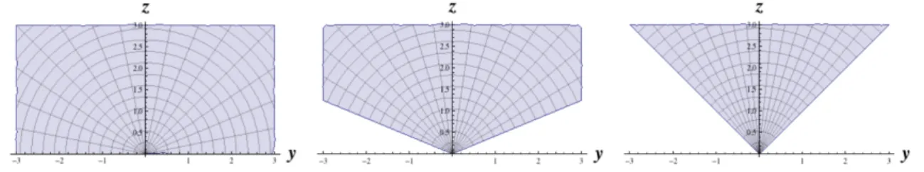
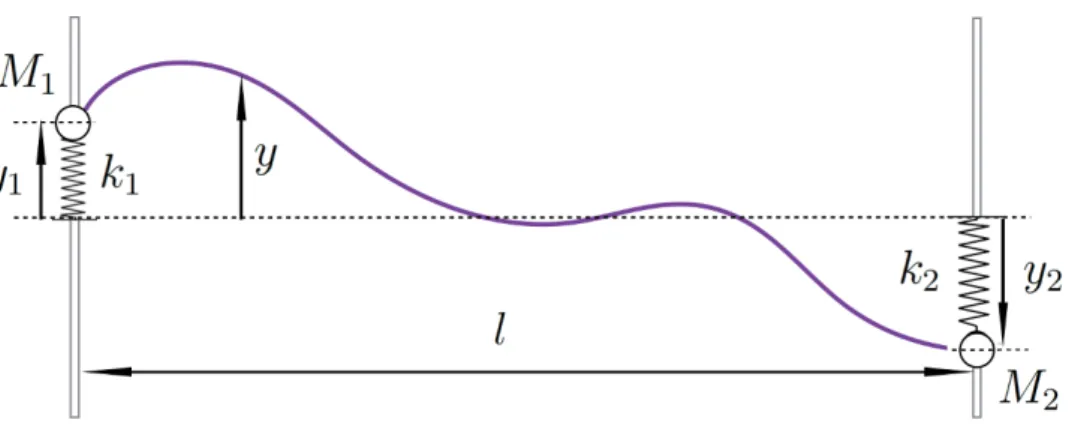
Figure 1. Anti-de Sitter waveguide: the left depicts a slice of AdS space in Poincar´e coordinates (y, z). In polar coordinates (ρ, θ), the AdS boundary is located atθ=±π/2(z= 0). The waveguide is constructed by taking the angular domain −α≤θ ≤+αforα < π/2, as in the middle figure.
For example, the waveguide for α=π/4 is given in the right figure.
this waveguide is embeddable to string theory: such geometry arises as a solution of Type IIB supergravity for nontrivial dilaton and axion field configurations and is known as the Janus geometry [21].
An important consequence of compactifying along non-isometry direction is the ap- pearance of the conformal factor cos12θ. One might try an alternative compactification scheme of AdS tube by putting periodic boundary condition that identifies the two bound- aries at θ= ±α. This is not possible. The vector ∂θ is not a Killing vector, so although the metric at hyper-surfaces θ = ±α are equal, their first derivatives differ each other.
We reiterate that the AdS waveguide is the unique choice for tunable compactification.
Another consequence is that the integration measure of the waveguide is nontrivial dVol(AdSd+2) = dVol(AdSd+1) dµd+2[θ] where dµd+2[θ] := dθ
(cosθ)d+2 (−α≤θ≤α).
(3.4) Before concluding this section, we introduce the notations that will be extensively used in later sections. We introduce the mode functions of AdS waveguide as follows:
Θs|Sn (θ) =n-th mode function for (d+ 1)-dimensional spin-scomponent that arise from (d+ 2)-dimensional spin-S field upon waveguide compactification. (3.5) Evidently, s = 0,1,· · · , S. We also introduce the first-order differential operators Ln
(n ∈ Z) of Weyl scaling weight n in the Hilbert space L2[−α, α] spanned by the above mode functions:
Ln= 1
` ∂θ+ntanθ
= 1
`(cosθ)n∂θ(cosθ)−n. (3.6) From the general covariance, it follows that all of ∂θ derivatives in the (A)dS wavegude are in the combination of these operators. So we will use Ln’s to express Kaluza-Klein normal-mode equations, gauge transformations and boundary conditions. As we will see, the Sturm-Liouville differential operator acting on spin-s field will carry the Weyl scaling weight (d−2s). The differential operator is quadratic in ∂θ, so acting on inner product of spin-s fields defined by the integration measure in eq. (3.4), Ln and Ld−2s−n are adjoint each other.
A comment is in order. In this paper, we mainly concentrate on AdS waveguide. How- ever, we can straightforwardly convert the results to the dS waveguide which we introduce
JHEP11(2016)024
in appendix C. The only technical difference is to replace (tanθ) to (−tanhθ), as can be seen in table 5. The spectral differential operators in dS are obtainable by changing the tangent functions in eq. (3.6).
4 AdS waveguide spectrum of spin-one field
In this section, we focus on the lowest spin field, spin-one, in AdS space and systematically work out Kaluza-Klein compactification on the Janus waveguide. In section 2, we learned that boundary conditions of different polarization fields are combined one another to fa- cilitate the Stueckelberg mechanism. In our AdS compactification, where the semi-direct product structure is the key feature, the choice of boundary conditions were left unspecified a priori. Here, we develop methods for identifying the proper boundary conditions. As this will be extended to higher-spin fields in later sections, modulo some technical com- plications (some of which actually open new physics), we will explain in detail how the boundary conditions are identifiable.
Through lower-spin examples, spin-one in this section and spin-two and spin-three in later sections, we shall compare two alternative but equivalent methods at the level of quadratic part of the action. One method is using the equations of motions, while the other method is using the gauge transformations. As the equation of motion contains increasingly complex structure for higher spin field (even at the linearized level), the first method is less practical for adopting to general higher-spin fields. The second method is relatively easier to deal with and can be applied to general higher spin fields. The second method has one more important advantage: the dimensionally reduced equations of motion can be derived by the second method. After compactification, the gauge transformations become Stueckelberg transformation. The point is that the Stueckelberg symmetries are as restrictive as the gauge symmetries (because the latter follows from the former, as we will show below), so it completely fixes the equations of motion for all massive higher-spin fields [15] to the same extent that the higher-spin gauge symmetries fix the equations of motion of higher-spin gauge fields. Therefore, it suffices to use the gauge transformations for obtaining information about the mass spectra of dimensionally reduced higher-spin fields.
For foregoing analysis, we use the following notations and conventions. The capital letters M, N,· · · will be used to represent the indices of AdSd+2: they run from 0 to d+ 1. The greek letters µ, ν,· · · are the indices of AdSd+1 space: they run from 0 to d. For the waveguide, index for the internal direction is θ. Therefore, M = {µ, θ}. The barred quantities represent tensors in AdSd+2 space, while unbarred quantities are tensors of AdSd+1. The AdS radius is denoted by`.
4.1 Mode functions of spin-one waveguide
We first consider the method using the equation of motion. The spin-one field equation in AdSd+2 space decomposes into two polarization components:
sec2θg¯M N∇MF¯µN =∇νFµν− Ld−2( L0Aµ−∂µφ) = 0, (4.1) sec2θ¯gM N∇MF¯θN =∇µ( L0Aµ−∂µφ) = 0, (4.2)
JHEP11(2016)024
where ¯AM = ( ¯Aµ,A¯θ) := (Aµ, φ). The (d+ 1)-dimensional fields Aµ, φ can be mode- expanded in terms of a complete set of mode functions Θs|1n (θ), labelled by the mode harmonicsn= 0,1,2,· · ·, on the interval θ∈[−α, α]:
Aµ=
∞
X
n=0
A(n)µ Θ1|1n (θ) and φ=
∞
X
n=0
φ(n)Θ0|1n (θ). (4.3) Mode functions are determined once proper boundary conditions are prescribed. As stated above, our key strategy is not to specify boundary conditions at the outset. Rather, we first require gauge invariance of various higher-spin fields and then classify all possible boundary conditions that are compatible with such gauge invariances.
What we learn from section2is that boundary conditions, equivalently, mode functions forAµand forφmust be related each other such that each term of eqs. (4.1) and (4.2) obey the same boundary condition. Otherwise, as we learned in section 2, equations of motion are accompanied with independent boundary conditions for each field and there would be no degree of freedom left after dimensional reduction. Therefore, each term of eq. (4.1) and eq. (4.2) must to be expanded by the same set of mode functions. We find that this consistency condition leads to the relations
0 Ld−2
L0 0
! Θ1|1 Θ0|1
!
= c01Θ1|1 c10Θ0|1
!
(4.4) among the spin-one modes and the spin-zero modes. Here,c01, c10’s are in general complex- valued coefficients. These equations reveals that the Sturm-Liouville (SL) operator −∆(s) in eq. (4.1) that determines the mass spectra of spin-one field in (d+ 1) dimensions is factorized to a product of two first-order elliptic differential operators,
Ld−2Θ0|1 =c01Θ1|1 and L0Θ1|1 =c10Θ0|1n . (4.5) We first note that L0 and Ld−2 are adjoint each other with respect to the measure eq. (3.4) for the field strength of (d+ 2)-dimensional spin-one field strength:
Z
dµd+2[θ](cos2θ)2A(θ)( Ld−2B(θ)) = Z
dµd+2[θ](cos2θ)2( L0A(θ))B(θ) (4.6) provided we impose Dirichlet boundary conditions at θ=±α. Acting L0 and Ld−2 to each equations of eq. (4.5), respectively, one obtains two Sturm-Liouville systems for spin-one and spin-zero modes,
spin-one Sturm-Liouville : ∆(1)Θ1|1 :=−( Ld−2 L0) Θ1|1 =−c11Θ1|1 (4.7) spin-zero Sturm-Liouville : ∆(0)Θ0|1 :=−( L0 Ld−2) Θ0|1 =−c00Θ0|1, (4.8) with the property that the eigenvalues of respective spins are paired up
−c11=−c10c01=−c00:=λ2. (4.9) Here, we took into account that L0 and Ld−2 are conjugate to each other and hence the eigenvalueλ2is positive semi-definite. This also puts the coefficientsc01, c10pure imaginary,
JHEP11(2016)024
and the eigenvaluesc00, c11 pure real. Hereafter, we label the eigenmodes in the ascending order of their eigenvalues and label them by n= 0,1,2,· · ·, viz. 0 ≤λ20 ≤λ21 ≤λ22 ≤ · · ·. The relations eq. (4.4) are then the statement that the SL spectrum is doubly degenerate:
for a spin-zero mode Θ0|1m for some m there ought to be present a spin-one mode Θ1|1n for somenproportional to Ld−2Θ0|1m , and for a spin-one mode Θ1|1m for somem there ought to be present a spin-zero mode Θ0|1n for somenproportional to L0Θ1|1m . By the aforementioned ordering of eigenmodes, we labeled the paired spin-zero and spin-zero modes by the same indexm=n= 0,1,2,· · ·.
Stated differently, the two first-order elliptic operators Ld−2, L0are not only conjugate each other but also act as raising and lowering operators between spin-one and spin-zero modes with doubly degenerate spectra
Θ1|1n
Ld−2 L0 with −λ2n=c11n =c00n =c10nc01n . Θ0|1n
(4.10)
As such, we refer to eq. (4.4), equivalently, eq. (4.10) as “spectrum generating complex”
for spin-one field in AdSd+2 space.
In fact, we can attribute such double-degeneracy to a hidden supersymmetry of the complex eq. (4.10).4 To see this, let us combine the two Sturm-Liouville problems for spin-one and spin-zero modes into one Sturm-Liouville problem acting on two-component modes
H
"
Θ1|1n
Θ0|1n
#
=
"
c11n 0 0 c00n
# "
Θ1|1n
Θ0|1n
#
, where H=
"
− Ld−2 L0 0 0 − L0 Ld−2
#
. (4.11)
Let us also introduce two supercharges Q=
"
0 0 i L0 0
#
and Q†=
"
0 i Ld−2
0 0
#
. (4.12)
Then, the two-component SL operator Hin eq. (4.11) is nothing but
H={Q,Q†}, {Q,Q}={Q†,Q†}= 0 (4.13) and the spectral relation eq. (4.4) is the statement that
Q
"
Θ1|1n 0
#
=ic10n
"
0 Θ1|1n
#
and Q†
"
0 Θ0|1n
#
=ic01n
"
Θ0|1n 0
#
, (4.14)
reinforcing the fact in eq. (4.6) that Ld−2 and L0 are conjugate to each other with respect to the inner product defined by the measure eq. (3.4). Moreover, the double degeneracy c11n =c00n is a consequence of the fact that the supercharges Qand Q† commute with the SL operator H.
4Note that the hidden supersymmetry is unrelated to the N = 2 spacetime supersymmetry of ten- dimensional Type IIB supergravity in which the Janus geometry is a classical solution that preserves half of the supersymmetry.
JHEP11(2016)024
Returning to the Kaluza-Klein compactification, the relations eq. (4.4) allow to de- compose the the (d+ 1)-dimensional field equations into spin-one and spin-zero modes as
X
n
h∇µFµν(n)+c01n (c10n A(n)ν − ∂νφ(n))i
Θ1|1n = 0 X
n
∇µh
c10n A(n)µ −∂µφ(n)i
Θ0|1n = 0. (4.15) We see that these equations take precisely the form of Stueckelberg coupling, triggering the Higgs mechanism for massive spin-one field in AdSd+1 space with mass
Mn2=−λ2n. (4.16)
Recalling the flat space counterpart in section 2, it may so happen that there exist massless — thus unHiggsed — spin-one or spin-zero fields in AdSd+1space. This is actually more interesting situation, so we would like to understand when and how this comes about.
Recalling that the SL eigenvalue is product of c10n and c01n and that the eigenvalue λ2n is positive semidefinite, there are three possible situations for the lowest eigenvalue:
(1) Doubly Degenerate Kaluza-Klein Modes: this case is when both ofc010, c100 are nonzero.
This implies that the spin-zero eigenvaluec00n and spin-one eigenvaluec11n are nonzero for all n = 0,1,2,· · ·. By the spectrum generating relations eq. (4.5), none of the corresponding modes Θ0|1n and Θ1|1n are annihilated by L0 and Ld−2, respectively. By the double degeneracy, the eigenvalue for spin-zero −c00n and the eigenvalue for spin- one −c11n are positive definite, and are paired up. The spectrum consists of doubly degenerate Kaluza-Klein modes. A special case is when bothc010 andc100 become zero.
In this case, the spectrum includes doubly degenerate ground modes. Nevertheless, we shall distinguish these two cases.
double Kaluza-Klein modes: L0Θ1|10 6= 0, Ld−2Θ0|10 6= 0
double ground modes: L0Θ1|10 = 0, Ld−2Θ0|10 = 0 (4.17) (2) Spin-One Ground Mode: this case is whenc100 →0 from the situation (1), leading to L0Θ1|10 = 0. This means that Θ1|10 is the ground mode with vanishing eigenvaluec110 = 0 of the spin-one SL operator Ld−2 L0. All higher modes, Θ1|1n for n = 1,2,· · · are necessarily massive. On the other hand, spin-zero eigenmodes Θ0|1n forn= 0,1,2,· · · have positive eigenvaluec00n >0. By the double degeneracy property, they are paired up with Θ1|1n forn= 1,2,· · ·. There is one spin-one ground mode of zero eigenvalue.
spin-one ground mode : L0Θ1|10 = 0, Θ0|10 = 0. (4.18) (3) Spin-Zero Ground Mode: this case is when c01 → 0 from the above situation (1), leading to Ld−2Θ0|10 = 0. This means that Θ0|10 is the ground mode with vanishing eigenvalue c000 of the spin-zero SL operator L0 Ld−2. All higher modes, Θ0|1n for n= 1,2,· · · are necessarily massive. On the other hand, spin-one eigenmodes Θ1|1n for
JHEP11(2016)024
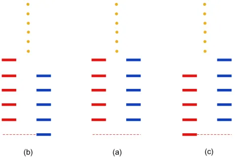
(b) (a) (c)
Figure 2. Various situations of double degeneracy between spin-zero (red color) and spin-one (blue color) modes. The middle spectrum (a) depicts the situation (1) that both c010 andc100 coefficients are nonzero. The spin-zero and spin-one modes are degenerate and have nonzero eigenvalues and so have no ground mode. The left spectrum (b) depicts the situation (2) thatc10→0. The spin-zero modes have no ground mode, while the spin-one modes have ground mode. The right spectrum (c) depicts the situation (3) that c01 →0. The spin-one zero modes have no ground mode, while the spin-one modes have ground mode. If both c010 and c100 are taken to zero, the spectrum is again doubly degenerate, but now starting from the ground mode.
n= 0,1,2,· · · have positive eigenvalue c11n >0. By the double degeneracy property, they are paired up with Θ0|1n forn= 1,2,· · ·. There is one spin-zero ground mode of zero eigenvalue.
spin-zero ground mode : Θ1|10 = 0, Ld−2Θ0|10 = 0. (4.19) These situations are depicted in figure2.
Remarks are in order. First, for the doubly degenerate modes of nonzero eigenvalues, if one of them is normalizable then the other is normalizable automatically. Thus, not only their eigenvalues but also their multiplicities also pair up. Second, the zero modes are solutions of the first-order differential equations L0Θ1|10 = 0 and Ld−2Θ0|10 = 0 subject to the Dirichlet boundary condition that render the two differential operators adjoint each other. As the measure dµ[cosθ] is nonsingular and as the interval [−α,+α] is finite, the existence of normalizable zero modes is always guaranteed.
We can classify the pattern of spectral pair-up by the elliptic index defined by I(s)=1 ≡X
n
Multiplicity(Θ0|1n )−X
n
Multiplicity(Θ1|1n )
= dim Ker Ld−2−dim Ker L0 (4.20)
JHEP11(2016)024
Here, we used the fact that all Kaluza-Klein modes n > 0 are paired up and so do not contribute to the index. In the situation (1), we have
c100 6= 0, c010 6= 0 : dim Ker L0 = 0 dim Ker Ld−2 = 0
c100 = 0, c010 = 0 : dim Ker L0 = 1 dim Ker Ld−2 = 1 (4.21) In the situations (2) and (3), we have
c100 = 0 : dim Ker L0 = 1 dim Ker Ld−2= 0
c010 = 0 : dim Ker L0 = 0 dim Ker Ld−2 = 1 (4.22) So we see that spectral asymmetry is present whenever the elliptic indexI(s)=1 is nonzero.
For the situation (1), the index is zero. For the situations (2) and (3), the index is nonzero.
Once again, the above results have close parallels to the supersymmetric quantum mechanics. A vacuum |vaci of supersymmetric system preserves the supersymmetry if Q|vaci = 0 or if Q†|vaci = 0. We see that the situations (2) and (3) preserves the supersymmetry, while the situation (1) preserves the supersymmetry only if the ground modes are present.
We can also determine the spectrum from the gauge invariances. In the waveguide, only those gauge transformations that do not change the boundary condition would make sense, viz. gauge fields and gauge transformation parameters ought to obey the same boundary conditions and hence the same mode functions. So, we have
δAµ=X
n
δA(n)µ Θ1|1n (θ) =X
n
∂µΛ(n)Θ1|1n (θ), (4.23)
δφ=X
n
δφ(n)Θ0|1n (θ) =X
n
L0Λ(n)Θ1|1n (θ) =X
n
c10n Λ(n)Θ0|1n (θ). (4.24) We see that the relations eq. (4.10), which was obtained by the method using the equation of motion, can now be derived by the variations eq. (4.24) and the Sturm-Liouville equations, eqs. (4.7), (4.8).
Putting together the field equations and the gauge transformations of n-th Kaluza- Klein modes, we have
∇µFµν(n)+c01n [c10n A(n)ν −∂νφ(n)] = 0
∇µ[c10n A(n)µ −∂µφ(n)] = 0 (4.25) δA(n)µ =∂µΛ(n)
δφ(n)=c10n Λ(n).
We recognize these equations as precisely the Stueckelberg equations of motion and Stueck- elberg gauge transformations that describe a massive spin-one gauge field (Proca field) in AdSd+1 space. Comparing them with the standard form of Stueckelberg system, we also identify the coefficients cn’s with the Stueckelberg coupling, viz. the mass of the Proca field, c10n =−c01n =Mn for all n >0.
The double degeneracy, as seen above, between spin-one and spin-zero fields is at the core of the Higgs mechanism, much as in the flat space counterpart in section 2. The
JHEP11(2016)024
Stueckelberg coupling that realizes the Higgs mechanism follows from two ingredients.
First, Kaluza-Klein modes of spin-one and spin-zero are coupled together, such that the second equation in eq. (4.15) follows from the first equation by consistency condition.
Second, the factorization property that the SL operator ∆(s)is a product of two first-order elliptic differential operators L0 and Ld−2 implies that the spectrum of spin-one mode is equal to the spectrum of spin-zero mode. The spin-zero mode provides the Goldstone mode to the massive spin-one (Proca) field when the mass of spin-one is zero, and this picture continues to hold in AdS space. A novelty for the AdS space is that the scalar field, despite being a Goldstone mode, is massive.
The double degeneracy and hence the Higgs mechanism breaks down for the ground mode. From eq. (4.15), we see that c01n, c10n are the Stueckelberg coupling parameters.
For the ground modes, either c010 , c100 or both is set to zero and so the corresponding Stueckelberg couplings vanish. In terms of the hidden supersymmetry, we see that inverse of the Higgs mechanism takes place whenever the supersymmetry is unbroken.
4.2 Waveguide boundary conditions for spin-one field
Having identified the mode functions as well as raising and lowering operators relating them, we are now ready to examine boundary conditions these mode functions must satisfy. To simplify and systematize the analysis, we shall first concentrate on boundary conditions which do not contain derivatives higher than first-order.5 In this case, all possible boundary conditions can be related to all possible choice of mode functions with nontrivial ground modes. This is because the ground modes eqs. (4.18), (4.19), which are valid everywhere in the waveguide θ = [−α, α], trivially satisfy the zero-derivative (Dirichlet) boundary condition and the one-derivative (Neumann) boundary condition, respectively, at θ=±α.
Moreover, by an argument similar to the reasoning around eq. (2.7) in flat space, we see that the situation in eq. (4.17) does not give rise to massless fields and that the situations in eqs. (4.18), (4.19) do give rise to massless spin-one and spin-zero fields, respectively.
So, to have massless fields in AdSd+1 space, we can choose the boundary conditions as (
Θ1|1|θ=±α= 0, Ld−2Θ0|1|θ=±α= 0 Dirichlet
L0Θ1|1|θ=±α= 0, Θ0|1|θ=±α = 0 Neumann (4.26) that give rise to massless spin-zero field and spin-one field, respectively, in AdSd+1 space.
The first corresponds to the situation that Θ0|1 is a zero mode belonging to Ker Ld−2 and the second case corresponds to the situation that Θ1|1 is a zero mode belonging to Ker L0. For each of the above two boundary conditions, the mass spectrum is determined by the Sturm-Liouville problem eq. (4.8). We emphasize again that the above choice of boundary conditions put all Kaluza-Klein modes to Stueckelberg coupling, leading to Higgsed spin-one fields. The ground mode of Dirichlet boundary condition, Θ1|10 (±α) = 0 has vanishing mass for spin-zero field and there is no massless spin-one field. The ground
5Fors≥2, as we shall show in next section, boundary conditions necessarily involve higher derivative terms in order to accommodate all possible mass spectra of higher-spin fields. In section 7, we discuss in detail origin and physical interpretation of higher-derivative boundary conditions (HDBC).
JHEP11(2016)024
Figure 3. Mass spectrum (Mn, s) for spin-one field in AdS waveguide. The left is for Di