Nonlinear Phenomena of Ultracold Atomic Gases in Optical Lattices: Emergence of Novel Features in Extended States

Review

Nonlinear Phenomena of Ultracold Atomic Gases in Optical Lattices: Emergence of Novel Features in Extended States

Gentaro Watanabe^1,2,3,4,5,*, B. Prasanna Venkatesh^4,6,7,* and Raka Dasgupta^4,8

1 Center for Theoretical Physics of Complex Systems, Institute for Basic Science (IBS), Daejeon 34051, Korea

2 Department of Physics, Zhejiang University, Hangzhou 310027, China

3 University of Science and Technology (UST), Daejeon 34113, Korea

4 Asia Pacific Center for Theoretical Physics (APCTP), Pohang, Gyeongbuk 37673, Korea

5 Department of Physics, Pohang University of Science and Technology (POSTECH), Pohang, Gyeongbuk 37673, Korea

6 Institute for Quantum Optics and Quantum Information, Austrian Academy of Sciences, Innsbruck A-6020, Austria

7 Institute for Theoretical Physics, University of Innsbruck, Innsbruck A-6020, Austria

8 Department of Physics, University of Calcutta, Kolkata 700009, India; [email protected]

* Correspondence: [email protected] or [email protected] (G.W.);

[email protected] (B.P.V.) Academic Editors: Ignazio Licata and Sauro Succi

Received: 16 December 2015; Accepted: 17 March 2016; Published: 31 March 2016

Abstract: The system of a cold atomic gas in an optical lattice is governed by two factors: nonlinearity originating from the interparticle interaction, and the periodicity of the system set by the lattice.

The high level of controllability associated with such an arrangement allows for the study of the competition and interplay between these two, and gives rise to a whole range of interesting and rich nonlinear effects. This review covers the basic idea and overview of such nonlinear phenomena, especially those corresponding to extended states. This includes “swallowtail” loop structures of the energy band, Bloch states with multiple periodicity, and those in “nonlinear lattices”,i.e., systems with the nonlinear interaction term itself being a periodic function in space.

Keywords:optical lattices; Bose–Einstein condensates; cold Fermi gases; superfluidity PACS:67.85.Hj; 03.75.Lm; 67.85.Lm; 03.75.Ss

1. Introduction

Following a long series of developments in the experimental techniques of atomic and optical physics, the Bose–Einstein condensation (BEC) of cold alkali atomic gases was realized in 1995 (see, e.g., [1–3] and references therein). The creation of this new state of quantum matter has opened up a new research field, the physics of ultracold atomic gases. The novelty of this system lies in its high controllability: various system parameters such as the dimensionality, the configuration of the external potentials, and the strength and the sign of the inter-atomic interaction can be manipulated dynamically as well as statically. In addition, this system has high measurability: since both the spatial and temporal microscopic scales of this system are relatively large, real time observation and direct imaging are possible. With these unique features, ultracold atomic gases serve as an unprecedented playground of the quantum world.

Due to the emergence of the superfluid order parameter, BECs acquire a nonlinear character originating from the interparticle interaction. Here, nonlinearity means that the basic equation governing

Entropy2016,18, 118; doi:10.3390/e18040118 www.mdpi.com/journal/entropy

the state of the system depends on the state itself. A variety of phenomena caused by nonlinearity such as solitons [4–7] and matter-wave mixing [8],etc. have been predicted and realized in BECs.

Remarkably, the strength of the nonlinearity in BECs of cold atomic gases is controllable. This is because heres-wave scattering lengthas, the parameter characterizing the interatomic interaction, can be tuned using the Feshbach resonance. Therefore, the realization of BECs of cold atomic gases has opened up a new horizon for the study of nonlinear phenomena (see, e.g., [9]).

With further development of technology and tools, superfluidity has been realized using cold fermionic atoms as well. It has been shown that, by increasing the interatomic attraction using Feshbach resonances, the state of an atomic Fermi gas can be varied in a controlled manner from a Bardeen–Cooper–Schrieffer (BCS) superfluid of delocalized Cooper pairs to a BEC of tightly-bound dimers [10]. Furthermore, these two limits are smoothly connected without a phase transition: the so-called BCS-BEC crossover [11–14]. The experimental confirmation of the BCS-BEC crossover is one of the prime achievements in the field of cold atomic gases. Using BCS-BEC crossover, we can understand both the Bose and Fermi superfluids from a unified perspective.

Another important development in the field of cold atomic gases is the realization of the external periodic potential called an “optical lattice”: Pairs of counter-propagating laser fields detuned from atomic transition frequencies, act as a free-of-defect, conservative potential for atoms via the optical dipole force. The realization of optical lattices has opened up the connection between the physics of cold atomic gases and solid state/condensed matter physics (see, e.g., [14–17] for reviews), and especially enables the simulation of theoretical models of solid state physics using cold atoms.

As a consequence of the competition and interplay between the effects of the periodic potential and nonlinearity, rich phenomena are expected to emerge in cold atomic gases in optical lattices.

Especially, equipped with Feshbach resonance, a knob for controlling the strength of the nonlinearity, cold atomic gases in optical lattices allow us to enter a regime in which the effect of the nonlinearity is comparable to (or even dominates over) that of the periodic potential. Such a strongly nonlinear regime beyond the tight-binding approximation has not been well-explored in conventional solid state physics. For example, a loop structure called “swallowtail” in the Bloch energy band [18,19] is a representative novel phenomenon emerging in this regime. In addition, using cold atomic gases, direct observations of the resulting nonlinear phenomena are possible, which is also a difficult task using solids.

In this short review article, we discuss nonlinear phenomena of superfluid cold atomic gases in optical lattices. Especially, we consider extended states and focus on the following phenomena: the swallowtail band structure, Bloch states with multiple periods of the applied optical lattice potential called multiple period states, and those in nonlinear lattices,i.e., systems with a periodically modulated interaction strength in space. This article is complementary to the existing review article on nonlinear phenomena in lattices [20], which focuses mainly on localized states. Superfluidity is the most important macroscopic quantum phenomena and superfluid flow in a periodic potential is ubiquitous in many other systems, such as superconducting electrons in superconductors and even in astrophysical environments such as superfluid neutrons in “pasta” phases in neutron star crusts (see, e.g., [21,22]

and references therein). Through the study of cold atomic gases in optical lattices, one may also expect to get deeper insights into these other systems.

This article is organized as follows. In Section2, we explain the setup of our system and basic theoretical formalism employed in the later discussions. In Sections3–5, we provide a comprehensive overview of the selected nonlinear phenomena in optical lattices starting with a simple physical explanation for each topic: swallowtail loops in Section3, multiple period states in Section4, and nonlinear lattices in Section5. Finally, summary and prospects are given in Section6.

2. Theoretical Framework

2.1. Setup of the System

In the present article, we discuss superfluid flows of either fermionic or bosonic atoms in the presence of the externally imposed periodic potentials. For the external periodicity, we mainly consider one of the most typical cases: one-dimensional (1D) sinusoidal potential of the form,

V(r) =V(x) =sERsin²qBx≡V0sin²qBx, (1) either in quasi-1D or 3D systems. Here,ER= ¯h²q²_B/2mis the recoil energy,mis the mass of atoms, qB =π/dis the Bragg wave number (note thatqBis different from the fundamental vector of a 1D reciprocal lattice, 2π/d, by a factor of 2), anddis the lattice constant,V₀≡sE_Ris the lattice height, andsis the dimensionless parameter characterizing the lattice intensity in units ofER. For simplicity, we also assume that the superflow is in the same direction as the periodic potential (i.e.,xdirection).

Throughout the present article, we set the temperatureT=0.

The systems which we discuss in this article consist of a large number of particles (the number of particles per site is also large) at temperatures close to absolute zero. One of the most convenient ways to deal with such many-body systems is to use the mean-field approximation. In this formalism, one focuses on a particular single particle, and the interactions produced by all the other particles are replaced by an averaged interaction described by the “mean field”. Thus the complicated many-body problem is effectively reduced to a far simpler one-body problem.

The mean-field theory provides a minimal framework to study the nonlinear phenomena emerging from the presence of the superfluid order parameter. The mean-field theory enables us to predict novel nonlinear phenomena and obtain qualitative understanding of them although its validity is not always guaranteed. We resort to a mean-field description throughout as it readily fits our motivation in the present review—to provide a physical explanation of some selected, novel nonlinear phenomena of superfluids in periodic systems.

In the rest of this section, we provide a brief explanation of the theoretical framework used in the discussions in the remaining part of this article. The main purpose of this section is to provide a minimal explanation and define the notation. Therefore, interested readers are encouraged to refer to other references (e.g., [1,2,13,23]) for further details.

2.2. Bosons

The mean-field theory describing Bose–Einstein Condensates (BECs) at zero temperature is given by the Gross–Pitaevskii (GP) equation [1,2,23–26]:

i¯h∂ψ(r,t)

∂t =

"

−^¯h

2

2m∇²+V(_r) +g|ψ(_r,t)|²

#

ψ(_r,t)_{. (2)} Hereψ(r,t)is the superfluid order parameter (or the condensate wave function) andgis the effective coupling constant between two interacting bosons given by

g= ^4π¯h

2as

m , (3)

whereasis thes-wave scattering length. The average number densitynis n= ^N

V = ¹ V

Z

|ψ(r)|²dr, (4)

whereNis the total number of particles andVis the volume of the system. Note that the GP equation can be viewed as the dynamical equation that results from a governing Hamiltonian known as the GP energy functional given by:

E[ψ] = Z

dr ¯h²

2m|∇ψ|²+V(r)|ψ|²+ ^g 2|ψ|⁴

!

. (5)

The stationary solution of Equation (2) is given by

µψ(r) =

"

−^h¯

2

2m∇²+V(r) +g|ψ(r)|²

#

ψ(r), (6)

whereµis the chemical potential.

Nonlinearity of the GP equation (the third term in the rhs of Equations (2) and (6)) originates from the interaction between bosonic atoms. Many previous studies have shown that GP equation describes BECs of dilute, weakly interacting bosons at zero temperature quite successfully (see, e.g., [23] and references therein).

2.3. Fermions

A useful method for treating superfluid Fermi gases is the standard BCS mean-field theory of superconductivity. Such a mean-field theory for inhomogeneous systems is given by the Bogoliubov-de Gennes (BdG) equations [13,27]:

H⁰(r) _∆(r)

∆^∗(r) −H⁰(r)

! u_i(r) vi(r)

!

=e_i u_i(r) vi(r)

!

. (7)

HereH⁰(r) =−^¯h

2

2m∇²+V(r)−µ. Also,vi(r)andui(r)are the quasiparticle amplitudes, associated with the probability of occupation and unoccupation of a paired state denoted by an indexi, whilee_iis the corresponding eigen-energy. The quasiparticle amplitudesv_i(_r)_andu_i(_r)satisfy the normalization conditionR

dr[u^∗_i(r)uj(r) +v^∗_i(r)vj(r)] =δ_i,j.∆is the order parameter (or the pairing field), which reduces to the pairing gap in the single quasiparticle spectrum in the region ofµ>0 for the uniform system. The pairing field∆(r) and the chemical potential µin Equation (7) are self-consistently determined from the gap equation,

∆(r) =−g

∑

i

ui(r)v_i^∗(r), (8)

and the average number density n= ^N

V = ¹ V

Z

n(r)dr= ² V

∑

i Z

|vi(r)|²dr. (9)

Since ∆depends on {ui} and{vi}, the BdG Equations (7) are nonlinear for nonzero interatomic interaction parameterg.

The superfluid Fermi systems bear a direct analogy with traditional superconducting systems, and likewiseg, the contact interaction, plays similar role as the weakly attractive interaction term in the BCS-model. Only, now gcan be both small or large, and its value can be externally tuned using Feshbach resonances by applying a magnetic or an optical field. This controllability leads to a crossover between two ends: a weakly attractive BCS-like superfluid and a condensate of tightly bound bosonic molecules of a pair of fermionic atoms; popularly called the BCS-BEC crossover [11,12].

For contact interactions, the right-hand side of Equation (8) has an ultraviolet divergence, which has to be regularized by replacing the bare coupling constantgwith the two-body T-matrix related to thes-wave scattering length [28]. A standard scheme [28] is to introduce a cutoff energyEc≡¯h²k²_c/2m in the sum over the BdG eigenstates and to replacegby the following relation:

1

g = ^m

4πh¯²as

−

∑

k<kc

1

2e⁽⁰⁾_k , (10)

withe⁽⁰⁾_k ≡¯h²k²/2m.

2.4. Discrete and Continuum Models

The systems of cold atomic gases can be studied by solving the GP equation (bosons) or the BdG equations (fermions) for the full continuum model. Let us, for the sake of simplicity, consider quasi-1D bosonic systems. So instead of V(r), we think of a potential in x direction only: V(x). If there is a periodicity in the form ofV(x), or, ifgitself is a periodic function ofx, one approach is to try the Bloch solutionsψ(x) =e^ikxφ(x)_{, where ¯}hk≡Pis the quasimomentum of the superflow and φ(x)is a periodic function with the same periodicity as the externally imposed periodicity byV(x)or g(x). One can expandφ(x)in terms of plane waves to give the following form for the order parameter:

ψ(x) =e^ikxφ(x) =e^ikx

lmax

l=−l

∑

a_le^i2πlx/d, (11)

to find the Bloch solutions. The normalization condition yields∑l|a_l|²=1.

Instead of going for the full solution, one easier approach is to map the system to a discrete model, borrowed from the idea of tight-binding model in solid-state physics. In this approach the density of bosonic/fermionic atoms is assumed to be concentrated around the minima of the optical lattice potential. For example, in a quasi-1D periodic potential, the condensate wave function can be approximated by a superposition of wave functionsφ_j(x)localized at the lattice sites, denoted byj, which are normalized asR

|φ_j(x)|²dx =1. Thus,ψ(x,t) = _∑jψ_j(t)φ_j(x). The coefficientψ_jis dependent on the site indexj.

The Hamiltonian for such a discrete model is H=−K

∑

j

(ψ^∗_jψ_j+1+ψ^∗_j+1ψ_j) +^U 2

∑

j

|ψ_j|⁴. (12)

In the case of the periodic solution with the same periodicity as that of the lattice (lattice constantd), the normalization condition is given by

Z d/2

−d/2|ψ(x)|²dx=ν, (13)

whereνis the filling factor (number of particles per site) with

ν=|ψ_j|². (14)

In evaluating the normalization condition, one neglects the overlap between φ_j’s localized at different sites.

The first term in the Hamiltonian describes hopping between the nearest-neighbor sites.

The hopping parameter Kis given byK = −R

φ_j[−_2m^¯h2∇²+V(x)]φ_j+1dx. The on-site interaction parameterUcharacterizes the interaction energy between two atoms on the same site, and gives the nonlinear term. ThisUis connected to the interatomic interaction parametergbyU=gR

|φ_j(x)|⁴dx.

In a manner similar to the continuum model one can also derive a dynamical equation for the

amplitudesψ_jfrom an extermisation of the energy functional corresponding to Equation (12). Such a dynamical equation is known in literature as the discrete nonlinear Schrödinger equation (analogous to Equation (2) for the continuous case) [29,30] and has served as an important tool to study ultracold atoms in optical lattices.

2.5. Energetic and Dynamical Stability

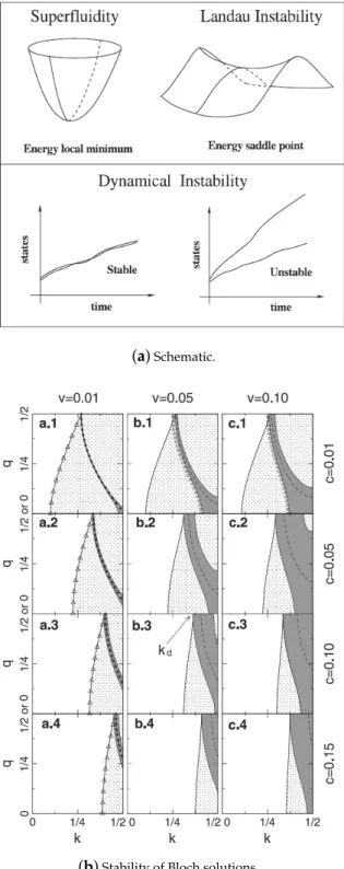
Once one can solve for the system, either from the full continuum model or the discrete version, the next step is to study the energetic and dynamical stability of the stationary solutions. Energetic stability guarantees that the stationary states are a local energy minimum of the energy functional (Equation (5)) and dynamical stability means that the time evolution of the system is stable with respect to small perturbations (this issue will be discussed in detail later in Section3.2.2). The standard approach in this context is the linear stability analysis described below [1,31–33].

Let δφq(x) be the deviation from the stationary Bloch wave solution φ(x) for a given quasimomentum ¯hkof the superflow. This can be written in the following form:

δφ_q=u(x,q)e^iqx+v^∗(x,q)e^−iqx. (15) Here ¯hqis the quasimomentum of the perturbation. The energy deviation from the stationary states can be written in the following form

δE= Z

dx

u^∗ v^∗

M(q) ^u v

!

. (16)

The matrixM(q)is Hermitian and gives the curvature of the energy landscape around the stationary solution. The system is energetically stable as long as all of the eigenvalues ofM(q)are positive. When even one of the eigenvalues is non-positive, the solution is no longer a local minimum and the system is energetically unstable. This is often termed as “Landau instability”.

For the same perturbationδφ_q, the time-evolution of the system for eachkis found to be:

i∂

∂t u v

!

=σ_zM(q) ^u v

!

, (17)

with

σz= ^{1 0} 0 −1

!

. (18)

Unlike M(q), the matrix σzM(q) is not Hermitian. If the eigenvalue ofσzM(q) is complex, the perturbation corresponding to an eigenvalue with positive imaginary part grows exponentially in time: in this case the stationary solution is dynamically unstable. If the imaginary part is zero, the stationary state remains stable (i.e., dynamically stable). Therefore, by noting the eigenvalues ofM(q) andσzM(q), one can learn whether the system belongs to an energetically stable region to start with, and how it evolves during the course of time. This is important because for BECs and superfluid Fermi gases, this stability translates to the sustenance of superfluidity in the system.

3. Swallowtail Loops in Band Structure

In this section we consider one unique manifestation of the nonlinearity (see Equation (2)) governing the dynamics of BECs in optical lattices—the so-called swallowtail loops in band structures. In the first Section 3.1 we provide the basic physical idea and the context in which swallowtail structures arise in the energy dispersions. Moreover, we discuss the key implication of having such swallowtail dispersions—breakdown of adiabaticity even at very slow driving. The purpose of this subsection will be to communicate the central physical picture

succinctly, hence we shall sacrifice chronology and use the most clear presentation (in our opinion) following [19,32,34,35]. In the second Section3.2we present a more detailed account of the various theoretical results on swallowtail band structures including their energetic and dynamical stability.

In the third Section3.3we present some experimental results that consider the effects of such nonlinear structures. In the following Section3.1, we present a brief account of more recent developments that extend the swallowtail phenomena to situations beyond the standards-wave interacting Bosons in optical lattices including dipole-dipole interactions, superfluid Fermi gases,etc. We conclude the section with some brief remarks indicating future prospects.

3.1. Basic Physical Idea: The Nonlinear Landau–Zener Model and Variational Ansatz for Condensate Wavefunction in Optical Lattices

The GP Equation (2) for the order parameter describing a BEC at zero temperature differs from the Schrödinger equation for a single particle in one key aspect — the presence of the interaction term g|ψ(r,t)|²in addition to the externally applied potential termV(_r). When the order parameterψ(_r)is expanded in terms of a given complete basis set of single particle wavefunctions, the nonlinear term in the GP equation essentially leads to an effective potential that is dependent on the occupation probability of the different single particle states. One may anticipate that in the limit that the nonlinearity is comparable to the external potential, i.e., gn ∼ V(_r), the resulting dynamics as well as the stationary solutions of the GP Equation (6) can be very different from the equivalent ones for the non-interacting g = 0 case which are simply governed by the eigen-energies of the Schrödinger equation.

The simplest model to see the structures that emerge in the limit of large nonlinearities is the nonlinear two-level system introduced in [34]:

i∂

∂t a b

!

=H(γ) ^a b

!

, (19)

H(γ) =

γ

2+^c₂ |b|²− |a|² v/2

v/2 −^γ₂−₂^c |b|²− |a|²

!

. (20)

Here γ gives the level separation and v/2 is the coupling between the levels. Withγ=αt, and g = 0, the above Hamiltonian is the well known Landau–Zener (LZ) model [36,37].

Equation (19) represents an extension of the LZ model representing the dynamics of a BEC with an order parameter whose overlap with the two relevant single particle levels has the amplitudeaandb.

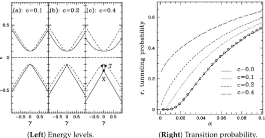
Let us now consider the main results of such a model. In the limit of the smallc=0.1, as shown in Figure1left, the adiabatic energy levels (or the chemical potentialµin the language of our theoretical framework) is qualitatively similar to the linear case with the characteristic avoided crossing. When the nonlinearity exceeds the coupling strengthv, the adiabatic energy levels are drastically changed with the development of the characteristic looped structures. Note that the shape of the loop for the chemical potential is not a swallowtail, the energy function has such a swallowtail structure.

While the modification of the energy level structure due to the strong nonlinearity is novel, what makes the looped energy structures particularly interesting from a physical point of view is the crucial implication of the looped structure for the transition probability between adiabatic energy levels.

In the linear case (c=0), the transition probability for the LZ model is given byr0=exp(−πv²/2α). In this case in the so-called adiabatic limit ofα→0, the transition probability vanishes. On the other hand in the nonlinear case, as shown in Figure1right, for strong enough nonlinearity such thatc>v there is a finite transition probability even in the adiabatic limit. A simple explanation for this behavior is discernible from the looped energy structure in the third panel of Figure1left—starting from the lower energy state initially, in the adiabatic limit there is very little tunneling as the system passes the point “X” and continues upwards along the loop to reach the final point “T”. At this point the system has to make a non-adiabatic transition to either the upper or lower level irrespective of how slow the

sweep rateαis. This breakdown of adiabaticity is the key implication as well as an indication of the loop structure arising from the nonlinearity.

(Left) Energy levels. (Right) Transition probability.

Figure 1.(Left) Adiabatic energy levels (or the chemical potentialµ) as a function of the nonlinearityc for the nonlinear LZ problem showing the emergence of loops forc>v. The dashed lines represent the adiabatic energy levels for thec=0 case. (Right) Tunneling probability as a function of drive speed αat different values ofc. For the linear case the result of the classic formular₀=exp(−πv²/2α)is displayed by the open circles. The figures are taken from [34].

Having captured the basic setting in which loops arise via the nonlinear LZ model, we move on now to the system central to this review—BEC in an optical lattice. We are interested in the stationary states of the GP equation that satisfy Equation (6). In analogy to the LZ model, when the nonlinearitygnis comparable to the applied lattice potential strengthV(x)we can expect interesting energy dispersions to arise. To be specific, henceforth we follow the treatment in [19,32] and consider a one-dimensional potential of the form:

V(x) =V0cos(2πx/d), (21)

and look for stationary states of the Bloch form, i.e., ψ(x) = e^ikxf(x) with f(x+d) = f(x). Here kdenotes the quasimomentum of the condensate and is the proper quantum number in a periodic system. A key quantity of interest is the energy per unit volume given by

E = ¹ d

Z d/2

−d/2dx

"

¯ h²

2m|∇ψ|²+V0cos(2πx/d)|ψ|²+ ^g 2|ψ|⁴

#

. (22)

In the absence of interactions, i.e., g = 0, the energy per unit volume is arranged into the usual band structure which repeats after every reciprocal lattice momentumk=2π/dand has gaps at the zone edgesk=_rπ/dwithran odd integer in the extended zone representation of the bands (or at k=±π/din the reduced zone schemes).

Equation (11) gives the full plane wave expansion for a Bloch state but a variational ansatz restricting to just three plane wave states,i.e.,lmax =1 can already capture much of the physics as shown in [32]. Since the relative phases of the plane wave amplitudes(a0,a1,a−1)do not change the energy, they can be chosen as real and using their normalization property restricted to the form:

a0=cosθ, a1=sinθcosφ, a−1=sinθ sinφ. (23)

The trial wavefunction (11) with the coefficients of the form (23) is inserted into the energy per unit volume expression (22) and extremized with respect to the parametersθandφ. Also the recoil energy E0=_¯hπ²_/2md²_(E0=_ERin the notation of this review article) serves as a convenient unit for different energies in the problem. Let us first consider the situation close to the Brillouin zone edgek=±π/d.

Using intuition from the nearly free particle models for periodic potentials, the ansatz (23) may further be simplified by takingφ={0,π/2}[19] giving:

ψ(x) =√ n e^ikx

cosθ+sinθe^−i2πx/d

(24) withnthe average particle density. In fact it was shown in [34] that such an ansatz can indeed be used to map the problem to that of the nonlinear LZ discussed earlier. At the zone edgek= π/d, upon extremization of energy density functional (22) yields the solutions cos 2θ= 0 or sin 2θ =_V0/(_gn)_. When gn < V0, the only possible solutions are θ = π/4 orθ = 3π/4 representing the zone edge solutions of the lowest and first excited band and are qualitatively similar to their counterparts in the linear,g=0, limit. The condensate current densityJ, given by the derivative of energyEwith respect tok, is zero for such solutions. When the interaction is strong enough such thatng >V0, the other solution withθ=sin⁻¹[V0/(gn)]/2 is also allowed. Moreover this solution has no linear counterpart and has non-zero current even at the zone edge with:

J=±^¯hπ md

s n²−^V

02

g² . (25)

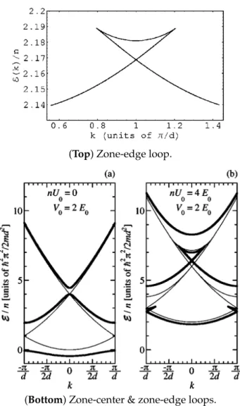
For values ofkaway from the zone edge with g > V₀/n, the two solutions originally located at θ=π/4 and sin⁻¹[V0/(gn)]/2 approach each other and finally merge giving rise to the typical loop structure depicted in Figure2top. Also note that the band-gap atk=π/din the weak lattice limit V0 E0is given byV0and the condition to have looped energy dispersion is that the interaction energy per particlegnbe greater than this band gap.

Remarkably, the variational trial wavefunction (24), withθvalues such thatE is extremized, is identical with an exact analytical solution found in [18,38]. While this initially leads one to suspect that loops are somehow a restricted phenomenon subject to the availability of such exact solutions, further work in [32] dispelled this notion by demonstrating the possibility of loops even at the zone center,i.e., withk=0, without any known exact solutions (see Figure2bottom). Such solutions are also captured by the variational ansatz (23). In this context the key solution in the linear limit is the one corresponding to the top of the second band withk=0 and energyE/n=4E₀per particle in the absence of interactionsg=0 andV0E0. This solution with an equal admixture ofa1anda−1, and very small contribution froma0hasθ=π/2 andφ=3π/4 (the solution withφ=π/4 corresponds to the third band now) persists even wheng6=0. However, it was shown in [32] that, for sufficiently large values ofg, this solution becomes unstable and two new solutions emerge signaling the lower and upper point of the loop atk=0 depicted in Figure2bottom. The condition for emergence of loops at the zone center is given by:

gn>(16E²₀+V₀²)−4E0. (26) In the weak lattice limit, the above condition simplifies togn>V₀²/(8E0)which is precisely analogous to the condition that interactions exceed the band gap similar to the criterion to have loops at the zone edge. Figure2bottom illustrates the zone-edge and zone-center loops computed using the ansatz (23).

Furthermore it was found in [32] that the size of the loops,i.e., their extent inkincreases monotonically as the ratiogn/V0is increased. Most interestingly in the limit of vanishing lattice potentialV0→0, the swallowtail loops extend over the entire Brillouin zone and the upper edge of the swallowtail becomes degenerate with the states in the bands above. As we discuss more in detail in the next subsection, this behavior stems from the fact that the states in the upper edge of the swallowtail correspond to periodic

soliton solutions of the GP equation in free space whose degeneracy is lifted by the application of a periodic potential.

(Top) Zone-edge loop.

(Bottom) Zone-center & zone-edge loops.

Figure 2.(Top) Swallowtail loop structure of the energy per particle as function ofkcomputed from the variational ansatz (24) forV0=3¯h(4V0/m)^1/2π/dandn=1.2V0/U0. Figure was taken from [19].

(Bottom) Energy per particle obtained using the variational ansatz (23) demonstrating the presence of swallowtail loops at both the zone edge and zone center for sufficiently strong nonlinearity.U₀in the figure isgin our notation. Moreover, the loops persist and extend over the entire band in the limit V₀→0. Taken from [32].

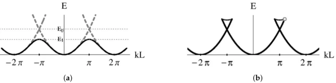
Finally, the swallowtail loop structures discussed so far may be intuitively viewed as generic features that arise in hysteretic systems as clarified in the work of [35]. Moreover the specific case of loops in the energy band structure of a BEC in an optical lattice can also be understood as a manifestation of superfluidity and extended to other analogous systems such as superfluids in annular rings that have been realized experimentally [39]. The key insight of [35] can be explained from Figure 3. In Figure3a, the approximately sinusoidal energy dispersion (lowest band) of a quantum particle in a periodic potential is shown. The corresponding Bloch eigenstates at different quasimomentum ¯hkhave periodic probability distributions commensurate with applied lattice potential. When a uniform external force is applied, the particle adiabatically follows this energy dispersion and performs periodic Bloch oscillations. In contrast for a BEC with interactions obeying the GP equation, i.e., a superfluid in a periodic potential, the interaction term tends to prefer uniform density distributions. Hence for strong enough interactions, as shown in Figure3b,

the adiabatic band structure tends to be more similar to the quadratic free particle dispersion.

This behavior has been referred to as the screening of the lattice potential by the superfluid in [35].

As a result, the velocity of the superfluid does not go to zero at the zone edge leading to non-zero current as expressed by Equation (25). As shown in Figure3b, the velocity cannot increase indefinitely and the dispersion terminates (gray circle in Figure3b) when the velocity becomes comparable to the Landau critical velocity of the superfluid giving rise to the swallowtail structure. Clearly adiabatic evolution along such a trajectory has to breakdown beyond this terminal point and forcing the system across this point from left to right and back will not restore the initial state—which is a clear sign of hysteresis. Also looking at the vicinity of the zone edge, it is clear that there are two possible minima for the energy which naturally leads to a saddle point separating the two minima given by the upper branch of the loop (the dotted lines in Figure3b).

(a) (b)

Figure 3.(a) The dashed line schematically shows the energy dispersion for a free particle which is modified to the solid line showing the (lowest) band structure on the application of a periodic potential of periodL. (b) Schematic plot of energy bands for a superfluid in an optical lattice that screens out the lattice to maintain non-zero flow velocity at the zone edge. Plots taken from [35].

The presence of multiple minima is a general characteristic of hysteretic systems. The number of minima for the superfluid in a periodic potential can be “controlled” by varying the quasimomentum

¯

hkor the interaction strengthgthat sets the size of the swallowtail loop (remember that the swallowtail loops disappear if the gis below some critical value). In the purview of catastrophe theory [40], which is the study of singularities of gradient maps (any physical theory where a generating function is minimized to identify the stationary states of the system such as Fermat’s principle in optics or the extremization of the GP energy functional here are examples of gradient maps), the swallowtail structures of energy bands represents a cusp catastrophe where two control parameters (gandk) may be varied to change the number of extrema of the energy by 2.

3.2. Swallowtail Loops Structures for Bosons in Optical Lattices

Having provided a physical picture of swallowtail loops in the previous subsection we proceed now to a comprehensive overview of the main results. We will divide this subsection into two parts.

In the first part we provide an account of the different results obtained regarding the occurrence of swallowtail loop structures for BECs in optical lattices and in the second part focus on the energetic and dynamical stability of the solutions.

3.2.1. Occurrence of Loop Solutions

The phenomenon of swallowtail loops in energy band structures arising from the GP equation were first investigated by Wu and Niu in [34] for the nonlinear LZ introduced in detail in the previous subsection. In this work it was also pointed out that the nonlinear LZ model naturally arises near the zone edge in the dispersion for a BEC in a periodic optical lattice potential. The key results from this pioneering work are noted in Figure1. Following this work, an exact solution for the GP equation in a periodic potential of the formV(x) = −V0sn²(x,κ)with sn(x,κ)denoting the Jacobian elliptic

sine function (with elliptic modulus 0≤ κ ≤ 1) was discovered in [38]. These solutions forκ =0 (Equation (2.1) of [18] or Equation (10) of [38] with elliptic modulusk=0 in their notation) take the following form in our notation:

ψexact(x) =

√c−v+√ c+v 2√

c e^iπx/d+

√c−v−√ c+v 2√

c e^−iπx/d (27)

withc=gn/(8E0)andv=V0/(8E0), which is of the Bloch wave form for the zone edgek=kL=π/d.

Whenc>v(which is also the condition for loops to appear at the zone edge), Equation (27) gives the solution with finite current (see Equation (25)).

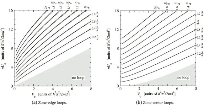
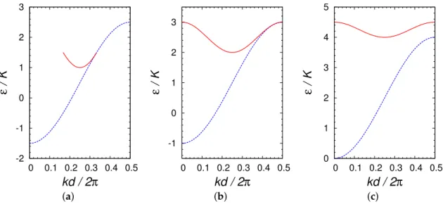
While on the one hand the exact solution lent more credibility [18] to the looped dispersions found from numerical solutions in [34], they also led to the suspicion that such solutions may not be a general feature. This was quickly dispelled by a simple variational calculation for the loops at zone edge by Diakonov et al. [19], followed by a more comprehensive analysis by Machholmet al.[32] demonstrating loops at the band center which we described in the previous subsection. Machholmet al.[32] also provided a thorough analysis of the width of the swallowtail loops, defined as the extent in quasimomentum space in an extended zone scheme, as the key parameters gn andV₀are varied for both the zone-edge loops (Figure4a) and zone-center loops (Figure4b).

(a)Zone-edge loops. (b)Zone-center loops.

Figure 4. Contour plot of width of swallowtail loops from a numerical minimization using the variational wavefunction (11) as a function of interaction (nU0isngin the notation of this review) and optical lattice depthV₀for zone-edge loops (a) and zone-center loops (b). Dashed lines in (a) are for truncation withlmax=2 and solid lines forlmax=3. Taken from [32].

The results in Figure4were calculated by a numerical minimization of the GP energy functional (5) with the ansatz (11). An unexpected feature of the results in Figure4is that the width of the swallowtail loops remain non-zero even in the limitV₀→0. In this limit the swallowtail solutions correspond to periodic soliton solutions of the GP equation. The zone edge solution withk=π/drepresents an equally spaced array of dark solitons (in one dimension, a dark soliton’s wave function vanishes at some point in space whereas for a gray soliton there is a density dip of non-zero value at some point in space) with one soliton per lattice spacingd. The wave number of the solutionk=π/dcan then be justified as the average phase change per unit length giving the right change in phase ofπacross

the dark solitons in each period. WhenV0 =0, soliton array solutions with density dips located at x=rdandx= (r+1/2)d(withrinteger) are degenerate and correspond to the highest energy state in the first band and the one immediately above in the second band, respectively. The lattice potential breaks this degeneracy as the solution with soliton centers at potential maximax =rdhave lower energy giving rise to the energy gap at the center of the swallowtail loop. The loops atk=0 can also be understood with an analogous argument. The solutions withk6=0 correspond to arrays of gray solitons. The phase change across a gray soliton is less thanπand they move with some finite velocity v_solitonin the absence of the potential. In order to create a stationary state from such solutions at finite V0, one has to imagine boosting the condensate velocity by−v_solitongiving a spatial dependent phase to the condensate wave function. The wave vector corresponding to such solutions now depends both on the density and the phase shift implied by the finite velocity boost. Moving away fromk=0 orπ/d, the minimum density andv_solitonincreases eventually going to zero and the sound speed (gn/m)^1/2respectively leading to the loop branch merging with the free particle dispersion as shown in Figure2bottom. This manner of understanding the emergence of swallowtail loop structures from the soliton solutions provides a complementary physical picture of the phenomenon.

The work by Mueller in [35] provides a general way to understand swallowtail loops from the point of view of hysteresis and superfluid response. A corollary of such an approach is that it is possible to extend the phenomena of loops to systems beyond the standard system in this review (BEC in a periodic potential). Amongst the various examples discussed in [35], the case of a BEC in an annular trap is of particular interest in the context of the experiment [39]. The Hamiltonian in the rotating frame describing a bosonic superfluid (massm) in a 1D ring of lengthL, rotating at a frequencyΩis

H

¯

h²/2mL² =

∑

j

(2πj+_Φ)²c^†_jc_j+^g˜

2

∑

j+k=l+m

c^†_jc^†_kc_lcm+λ

∑

j

c^†_jcj−1+c^†_jc_j+1

. (28)

In the above, cj stands for the annihilation operator for bosons with angular momentum j¯h in a quantized picture or the amplitude of occupation of the same mode within a mean-field GP-like picture,Φ=2mL²Ω/¯his the rotation speed in a dimensionless form, ˜g=4πasL/d²_⊥is the effective interaction for a trap perpendicular to the ring with harmonic oscillator lengthd⊥, andλis an impurity term that breaks the rotational symmetry coupling different angular momenta. This can arise naturally due to imperfections in the container or be generated, for instance, by applying a laser potential externally. The key point is that there is a one-to-one correspondence between the Hamiltonian (28) and the GP energy functional (5) after substituting the Bloch ansatz (11) withΦplaying the role of quasi-wave numberkandλplaying the role of the periodic potential strength leading to swallowtail loops as shown in Figure 11 in [35]. We will revisit Equation (28) in Section3.3. Seamanet al. [41]

and Dong and Wu [42] provided an interesting insight into the swallowtail loop structures for both repulsively (g>0) and attractively (g<0) interacting BECs for the special case of a Kronig–Penney periodic potential which is of the form,

V(x) =V₀

∑

δ(x−jd)_{. (29)}

The Bloch states in such a potential can be solved analytically. For the repulsive interactions case, the results in [41] agreed qualitatively with the earlier numerical and approximate calculations but had unique features such as the fact that the critical interaction strength to have loopsgn>2V0for allbands of the energy spectrum unlike the sinusoidal band case discussed in [32]. In the case of attractive interactions withg<0, they found the loop structures occurred in the upper branch at the band gaps, starting from the second band as shown in Figure5. Moreover for the strongly attractive casegn=−10E0shown in Figure5the loop in the second band spans the entire Brillouin zone and splits from the original band.

Figure 5.Energy bands with swallowtail loops in the excited bands for a Kronig–Penney potential (Equation (29)) withV₀=E₀and attractive interactiongn=−10E₀. Taken from [41].

3.2.2. Stability of Loop Solutions

In the discussion of swallowtail loops so far, we have completely ignored the stability properties of the solutions. In what follows, we discuss results regarding the energetic and dynamical stability of steady state solutions of the Bloch form (of which swallowtail loops are special cases) for BECs in periodic potentials. The stability of the solutions we find by extremizing the GP energy functionals (5) are crucial as they will provide us clues as to whether in an experiment the system can reach such equilibrium solutions and if they do how long can they be stable. As a part of the the theoretical framework Section2.5, we provided the conditions for energetic stability but a physical picture of the two kinds of stability as exemplified in Figure6a is helpful—for energetic stability the equilibrium solution has to be a local minimum of the energy functional (5) whereas for dynamical stability perturbations about the equilibrium state should not grow with time when evolved according to the time-dependent GP Equation (2).

The stability of Bloch states in the lowest band excluding loops was discussed by Wu and Niu in [31] and [43]. Figure6b represents the results from a numerical calculation mapping out the stability of Bloch states with quasimomentum ¯hkunder perturbations of the Bloch wave form with quasimomentum ¯hqfor different values of the potentialv=V₀/(8E₀)and nonlinearityc=gn/(8E₀)_. Let us denote the stability matrix, Equation (16), for a state with quasimomentum ¯hk under a perturbation of quasimomentum ¯hqas M_k(q). For the special case of a free BEC with no lattice, i.e., v = 0, the eigenvalues of the matrix can be computed analytically and the requirement for positivity of eigenvalues leads to the well-known Landau criterion given by

|k| ≥ q

q²/4+c. (30)

The shaded light and dark regions in Figure6b represent regions of energetic instability withMk(q) having negative eigenvalues. In the limit of smallvthe equality in the expression (30) accurately reproduces the energetic stability region shown by triangles in the plot. Another key feature to note in Figure6b is that even atvcomparable toc, as the nonlinearitycis increased, the BEC is energetically stable over an increasing area in thek-qspace, which can be anticipated from expression (30).

(a)Schematic.

(b)Stability of Bloch solutions.

Figure 6. (a) Schematic illustration of the physical principle behind the definitions of energetic and dynamical stability. A dynamically unstable state is always energetically unstable whereas the vice-versa is not true. (b) Stability phase diagram at different values of lattice depth and nonlinearity parameter for a BEC in an optical lattice. The relation between the notation in the picture and this review article is scaled potentialv=V₀/(8E₀)and nonlinearity parameterc=gn/(8E₀).qis the wave number of the perturbation modes andkthe quasimomentum in units of 2K=4π/d. In the shaded dark and light areas the system is energetically unstable while in the shaded dark area it is dynamically unstable. Triangles in (a.1–a.4) represent the boundaryq⁴+c=k²expected forv=0 and full dots in first column are from the results of an analytical calculation using Equation (31) valid forv1.

Broken curves indicate the most unstable modes for each quasimomentum. The open circles in (b.1) and (c.1) represent analytical result valid forcv(see Equation (5.14) of [43]). Figure taken from [43].

In Figure6b, the system is dynamically unstable in the dark shaded regions. The first thing to notice is that energetic instability is a pre-requisite for dynamical instability and this can also be shown in general (see appendix of [43]). Further insight into dynamical stability can be obtained by considering the structure of the eigenvalues of the matrixσ_zMk(q)since the requirement for dynamical stability is to have real eigenvalues for this matrix. The states represented by the eigenvectors of σzM_k(q) can also be viewed as quasiparticle excitations in the BEC, i.e., phonons [43], with the positive eigenvalues giving the phonon spectrum. In general the eigenvalues of σzMk(q) can be complex but always occur in complex conjugate pairs [32,43] owing to the real nature of the matrix in momentum representation. In the case ofv =0, the eigenvalues ofσzM_k(q)are always real and given bye±(q) =kq±^pq²c+q⁴/4 wherekandqare measured in units of 4π/d. This implies that in free space BEC, flows are always dynamically stable. However, Figure6b shows that situations change significantly when the lattice potential is introduced as also evidenced in experiments [44–46].

In general for all parameter regimes there is a critical wave numberk_dbeyond which Bloch waves are dynamically unstable. Atk=k_d, dynamical stability always sets in forq=π/d, which interestingly also corresponds to a period doubling revealing a link further explored in Section4. At the point where dynamical instability sets in, the eigenvalues ofσzM_k(q)change character from real to pairs of complex conjugates,i.e., with equal real parts. Hence as explained in [31,32,43], dynamical instability can be viewed as arising from a lattice induced resonance between a pair of excitations that are degenerate in thev=0 limit. Thus when the instability sets in, two phonons with the sum of their momenta given by the primitive reciprocal lattice vectors±G=±2π/dare created from zero energy,i.e., they satisfy e+(q) +e+(2π/d−q) =0 . (31) This can be used to clearly justify the observation (valid at small lattice depthsV₀) that instability at the critical wave numberkdalways sets in withq = G/2 = π/dand the critical vector satisfies

|k_d|= (π/d)(gn/2E0+1/4)^1/2agreeing with the numerical results in Figure6b.

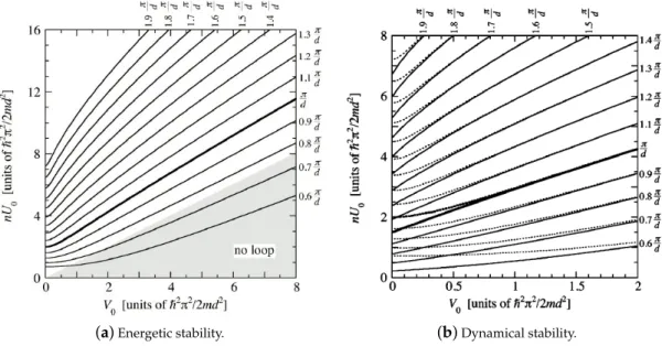
In the stability analysis of [32], in addition to standard Bloch states, also the ones corresponding to the loop solutions (lower branch) were considered. In Figure7the results of this analysis is shown by plotting the largest Bloch wave vectorkfor which the states are energetically stable as a function ofng andV0. States with 0≤k≤π/dcorrespond to states with the lowest energy andk>π/drepresents lower edge-loop states. In general it was found that the range of quasimomentum values at which the system is energetically stable increases with the interaction strengthgn. They also found that the wave vector of the tip of the swallowtail sets a natural limit for the wave vector at which instability sets in for parameter regimes where swallowtail loops occur. Moreover they found, in agreement with [31], with increasingkthe long wavelength perturbations withq→0 become energetically unstable first.

Hence a hydrodynamic description can be constructed [47–49] and it also gives analytical predictions for the instability contour as a function ofV0andgnfor the zone edge withk=π/dwhich compares favorably with the numerical calculations [49]. Note that as expected the states on the upper edge of the loop are always energetically and dynamically unstable.

Finally, the discussion so far was limited to only the linear stability of equilibrium solutions but the full response of the solutions of time dependent GP Equation (2) to perturbations was also studied numerically in [41]. Here the stable lifetime of a given initial equilibrium state was defined as the time taken for the variance of the Fourier spectrum of the time-dependent order parameter from the initial Fourier spectrum (normalized to the initial spectrum) to exceed the value 1/2,i.e., the time at which the order parameter becomes very different from the initial solution and taken as an indicative time for onset of dynamical instability. They found that for weakly attractive condensates the zero quasimomentum Bloch state in the first band is long-lived under white noise perturbations but highly unstable for time periodic perturbations. For both weak and strong attractive interactions the higher band Bloch states are unstable but the first band Bloch states with non-zero quasimomentum can be stable even to harmonic perturbations owing to their negative effective mass (defined as the inverse of the Band curvature). For weak repulsive interactions, Bloch states in the

lowest band are stable as long as the quasi-wave numberk<π/d, as at larger quasi-wave numbers the effective mass becomes negative, for the particular choice of Kronig–Penney potential (29) used in [41]. However, in agreement with the linear stability analysis, as the interaction strength grows, larger parts of the energy band including the lower branch of the loops are stable. In a later publication the same authors [50,51] showed that there is always a small part of the loop in the repulsive case that has negative effective mass but this area’s extent monotonically decreases asgnis increased.

A clear discussion of the dynamical stability of attractive BECs in an optical lattice is provided in [52].

A recent review [53] also provides detailed treatment of stability of BECs in optical lattices.

(a)Energetic stability. (b)Dynamical stability.

Figure 7. Contour plot of maximum quasimomentumkfor energetic stability (a) and dynamical stability (b) as a function of interaction and lattice depth for zone-edge loops.k≤π/drepresents states on the lowest branch of the ground band andk>π/dthe states on the lower edge of the swallowtail loop. The dashed lines in (b) are energetic stability curves for comparison. Taken from [32].

3.3. Experimental Realization

In the past decade and half there has been tremendous progress in the field of ultracold atoms in optical lattices [14,15] with a range of experiments tackling interesting many-body physics. In this light it must be said that specific experiments dealing with nonlinear energy dispersions in optical lattices have been few and far in between.

The earliest relevant experiment concerns the instability of superfluids in optical lattices by the group at LENS, Florence reported in Burgeret al. [44–46]. In this experiment a cigar shaped quasi-1D BEC was localized in an harmonic trap and an optical lattice potential was also turned on.

Following this, the center of the trap was suddenly shifted, corresponding to a sudden change of the quasimomentum in our language. For small shifts∆xthe dynamics of the BEC was coherent but for shifts greater than a critical value∆x>_∆xc, the oscillations are disrupted and the dynamics became dissipative. The authors of the experiment attributed this to the energetic Landau instability of the condensate. But theoretical work from Wu and Niu [43,45,46] showed that it may be more appropriate to associate this behavior with dynamical instability especially considering that the experimental parameters fall in a regime (c∼0.02,v∼0.2) where dynamical instability is rampant (see Figure6b) and the critical displacement∆xc increases with decrease of lattice depth in the experiment (the energetic stability is essentially independent of lattice depth in the linearized stability treatment).

A follow-up comment from the authors of the experiment [45,46] was essentially inconclusive but hinted that even the GP equation may not be a valid description for some of their experimental results and beyond mean-field effects may have to be included. Following this, in [54] a thorough theoretical

treatment of the problem including 3-dimensional GP equations and effective 1-dimensional GP equations taking into account the transverse degrees of freedom was undertaken. This theoretical treatment adapted to the experiment [44] clearly showed that the onset of instability observed in the experiment was due to dynamical instability. There are two main reasons that led to some uncertainty regarding the conclusions in the experiments [44]—the inability to distinguish experimentally between dynamical and energetic stability as both processes manifest as an enhanced loss of atom number from the condensate and the inability to accurately set the initial quasimomentum of the condensate as a mean displacement from the harmonic trap center can in general lead to a mixture of quasimomenta and band eigenstates.

In the follow-up experiment from the LENS group [55,56] both these issues were succesfully resolved. In [55], a moving optical lattice was implemented by frequency detuning the two laser beams creating the lattice. The ground state in a moving lattice is simply a state with a finite quasimomentum.

By varying the amount of detuning, they were able to load the BEC adiabatically into states with a given quasimomentum both in the ground and excited bands. A subsequent measurement of the loss rates as a function of quasimomentum revealed a threshold for the onset of dynamical instability in very good agreement with the theoretical expectation for the lattice depth used. In [56] they were able to also distinguish between the onset of energetic and dynamical instability by an ingenious use of a radio-frequency (RF) shield to selectively control the thermal fraction of the atomic cloud. The presence of the thermal cloud can effectively trigger energetic instability, which has generally a lower threshold in quasimomentum, by providing a dissipation channel. Hence when a large thermal fraction is present, the onset of dynamical instability is marred by energetic instability. On the other hand when the RF shield is turned on to remove the thermal fraction and experiments are performed with nearly pure condensate, the onset of dynamical instability stands out via a dramatic loss of atom number. It is important to emphasize at this point that experiments such as [44] are performed at small lattice depths v. In this regime, as evident from Figure6b, there are significant regions of quasimomentum space that are energetically unstable but dynamically stable. On the other hand at large lattice depths (see Figure 1 of [56]), the region of quasimomentum space that exhibits only energetic instability is tiny. Thus in this so called tight-binding lattice limit, there was unambiguous agreement between experiments [57]

and the theoretical [43,58] and numerical [59,60] treatments that predicted dynamical instability.

It was also shown in [58] that the dynamical instability in this regime can also be viewed as a kind of modulational instability which is a general feature of nonlinear wave equations where a small perturbations of a carrier wave can exponentially grow as a result of interplay of dispersion and nonlinearity.

In [61], the behaviour of the critical quasimomentum upto which superfluidity persisits across the superfluid-Mott insulator (SF-MI) quantum phase transition was studied. Within a mean-field GP picuture, as we have discussed in Section3.2.2, the stability of the superfluid is in general enhanced with increasing interaction and lattice depth. On the other hand, within the full quantum model, there is a critical interaction strength to tunneling ratio beyond which the system is no longer superfluid and goes into the Mott insulating phase where the critical quasimomentum is trivially equal to 0.

This study maps the behaviour of the critical quasimomentum as it goes from a finite value in the SF phase to zero in the MI phase giving an accurate determination of the phase boundary. In [62] beyond dynamical instability at the zone edge is investigated experimentally and theoretically within the truncated Wigner approach which can account for beyond GP effects including the thermal depletion of the condensate. Finally, in recent experiments [63] dynamical instability of spin-orbit coupled (SOC) BECs in moving optical lattices was investigated and a manifestation of the breakdown of Galilean invariance predicted for SOC systems was evidenced by the difference in the strength of the dynamical instability (measured by atom loss rate) depending upon the direction of motion of the lattice.

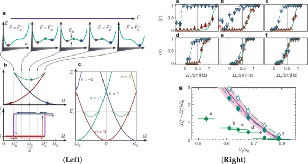
In the seminal experiment of the Bloch group [64], some aspects of the nonlinear LZ tunneling phenomena originally considered in the theoretical work of Wu and Niu [34] was explored.

The experimental system consisted of an array of tubes of BECs in a 2D optical lattice potential.

A superlattice potential alongxdirection allows pair-wise coupling between tubes giving many copies of coupled double wells. In the experiment they effectively realize the nonlinear LZ energy function of the the form:

E[ψ_R,ψ_L]≈ ^∆ 2

|ψ_R|²− |ψ_L|²−J(ψ^∗_Rψ_L+c.c.) +^U

2hδnˆ²i|ψ_R|⁴+|ψ_L|⁴, (32) whereψ_Landψ_Rrepresent the amplitude to occupy either the left or the right tube. ∆, the energy detuning between the tubes, andJ, the tunnel coupling between the tubes can be controlled by varying the relative phase and lattice depth respectively of the superlattice potential alongxdirection.

The experimental protocol consists of preparing all the atoms initially in the left tube with the initial detuning∆ieither chosen to be negative (ground state) or positive (excited state) and sweeping the detuning at the linear rateαand finally measuring the number of atoms in the left and right tube.

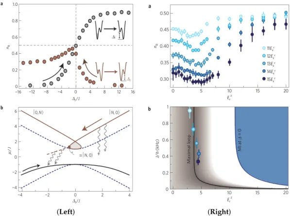
As already anticipated by Wu and Niu [34], the model (Equation (32)) is exactly the same as the one introduced in Equation (19) except for the interaction term’s sign is switched. As a result once the ratio of interaction to tunnelingη=_Uhδnˆ²i/J(c/vin [34]) is large, there is a loop in the upper branch as shown in lower panel of Figure8left. In the experiment, for sweeps along the ground state branch (gray dots in Figure 8left) there is no adiabaticity breakdown observed. In the sweep starting with the excited state (left tube at higher energy), there is a complete breakdown of adiabaticity even for reasonably small sweep ratesα(red dots in Figure8left). Moreover, for small sweep rates the transfer efficiency, given by number of atomsnR in the final state, decreases with decreasing sweep rate completely opposing the expected LZ behavior. The presence of the loop in the upper branch contributes to this adiabaticity breakdown for small sweep rates, as the atoms follow the upper branch and are self-trappedin the middle branch of the loop, (see lower panel of Figure8left) which is a local maxima.

They finally make a diabatic transition to the adiabatic ground state at the loop edge leading to the sharp breakdown of transfer efficiency near zero detuning seen in Figure8left upper panel. A confirmation of the effect of loops on the adiabaticity breakdown is provided by the non-monotonic behavior of the transfer efficiency (number of atoms in the initially empty right tube at the end) at a given sweep rate and tunnel coupling as a function of thez-lattice depth shown in top panel of Figure8right.

At smallz-lattice depths, an increase in lattice depth effectively increases the on-site interactionUhδnˆ²i, leading to larger loop sizes which leads to lower transfer efficiency but eventually beyond a certain lattice depth the suppression of on-site fluctuationshδnˆ²i dominates leading to a decrease in the effective interaction and increase of transfer efficiency restoring standard LZ behavior. Moreover as shown in the lower panel in Figure8right, the experimentally determined minimum transfer efficiency agrees with a theoretical calculation for the position of the maximum loops size as a function of the z-lattice depth and tunnel coupling.

In the experiment by Eckelet al.[39], a physical situation approximately corresponding to the Hamiltonian in Equation (28) was realized for a BEC of²³Na atoms confined in a ring shaped trap.

The goal of this experiment was to observe hysteresis between quantized states of circulation of the superfluid BEC caused by the presence of swallowtail loops in the energy landscape of such a system [35,65]. In the experiment [39], they were concerned with the quantized circulation states with winding numbersn =0 andn =1 with frequencyntimes the rotational quantaΩ0 =¯h/mR²and drive transitions between these states by tuning the relative angular velocity between the trap and the superfluidΩwhich can be controlled by applying a repulsive rotating laser potential.