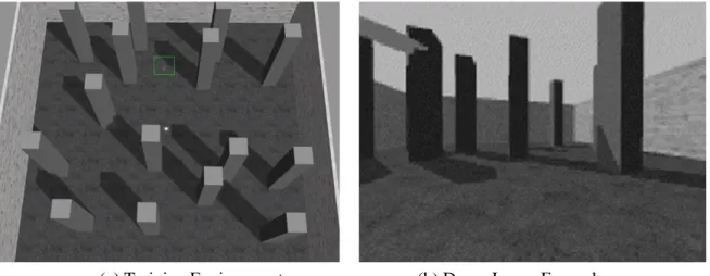
Autonomous navigation of unmanned aerial vehicles (UAVs) has posed several challenges due to the limitations regarding the number and size of sensors that can be attached to the mobile robots. Although sensors such as LIDARs that directly acquire distance information from the surrounding environment have proven to be effective in avoiding obstacles, the weight and cost of the sensor add to the limitations of use for UAVs as recent trends require smaller sized UAVs. Conventional methods regarding visual navigation make use of features within the image data or estimate the depth of the image using various techniques such as optical flow.
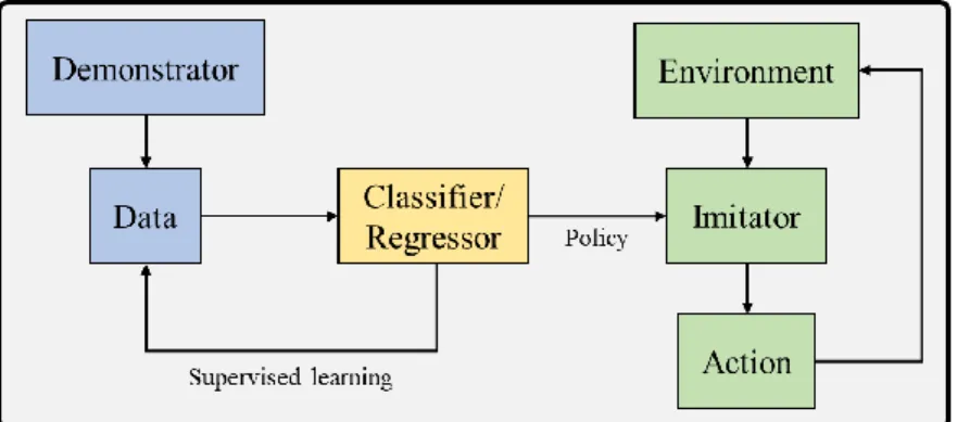
A newer approach to vision-based obstacle avoidance utilizes heuristic methods based on artificial intelligence such as deep learning technologies, which have shown state-of-the-art performance in areas such as image processing or voice recognition. Such heuristic methods have been shown to be more efficient as the rules and features drawn from the image are automatically determined, as opposed to conventional methods where the rules and features are explicitly determined by humans. In this thesis, we propose an imitation learning framework based on deep learning technologies that can be used for obstacle avoidance by UAVs, where the neural networks in this framework are trained on flight data obtained from human experts, and extract the necessary features and rules. to perform certain tasks.
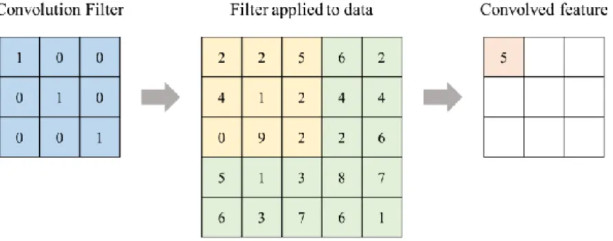
A CNN (Convolutional Neural Network), 3D-CNN and a DNN (Deep Neural Network) will each be applied to the framework and tested with respect to collision ratios to validate its obstacle avoidance performance.
INTRODUCTION Motivation
Research Objectives
Through the implementation of this communication node, we can not only test and evaluate the proposed system, but also expect future use of the system in actual systems. The second goal is to develop a deep learning model capable of extracting the necessary spatial features and deriving a certain rule on the training dataset. Unlike most conventional obstacle avoidance studies, the proposed neural network in this study will heuristically extract the features and obtain a certain obstacle avoidance rule.
Under the main assumption that there is some underlying relationship or function between visual input and actions of a human when it comes to obstacle avoidance, we focused on teaching an agent to map visual inputs to the guidelines for obstacle avoidance. Through sufficient acquisition of camera data and the corresponding control inputs generated from human experts, our neural network is likely to learn the underlying obstacle avoidance rule. In this paper, we present a framework for obstacle avoidance with deep learning-based imitation learning methods.
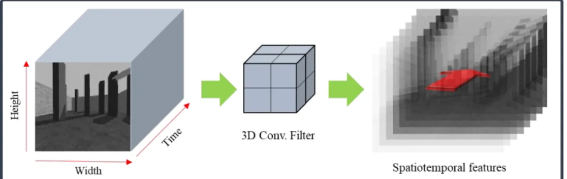
3D-CNN models [Learning spatiotemporal features with 3d convolutional networks] will be used for the imitation learning framework, since obstacle avoidance with a monocular camera is considered a sequential task.
Outline of the Thesis
LITERATURE REVIEW
Conventional Obstacle Avoidance Methods
Heuristic Obstacle Avoidance Methods Reinforcement Learning
DEEP NEURAL NETWORKS Artificial Neural Network
Activation Function
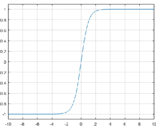
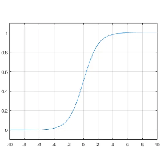
The hyperbolic tangent function has a sigmoidal shape similar to the sigmoid function, but the output values are between the range -1 and 1. Such properties reduce the probability of the network getting stuck during the training phase as the range increases from (0, 1) to (-1, 1 ). The Rectified Linear Unit (ReLU) function is another type of activation function used for neural networks.
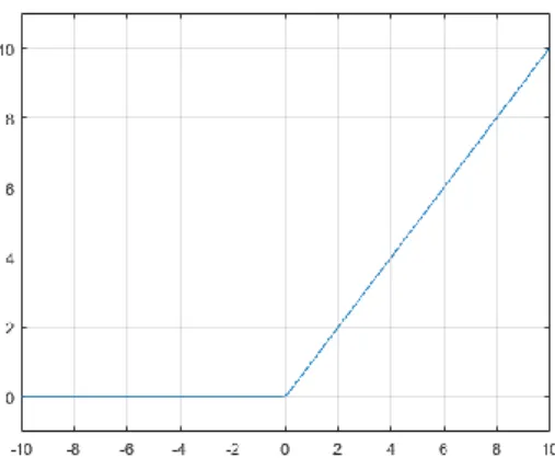
In response to the learning rate or weight update problem for the sigmoid function, the ReLU function has been widely adopted as it uses only positive output values. The main advantage of this function is that the gradient is either 0 or 1, overcoming issues such as the vanishing gradient problem.
Backpropagation
Convolutional Neural Network
Convolution Layer
Pooling Layer
Fully Connected Layer
3D-Convolutional Neural Network
IMITATION LEARNING-BASED OBSTACLE AVOIDANCE FRAMEWORK Problem Statement
Data Acquisition and Preprocessing
One corresponding control input from the human expert was stored in the database with a time stamp so that it could be linked to the image data during the training process. For simplicity, a total of three directions were used: left, right, and straight, and the control input directions were applied to the drone incrementally, so that the drone's heading angle increases or decreases depending on the size or duration of the drone. previous control input directions. One-hot encoding was applied to the control input data before the training process was completed.
One-hot encoding is a way of encoding categorical integer features into a one-hot numeric array [29], which is widely used in machine learning in many cases where categorical variables do not have an ordinal relationship. After the training data was completely collected, the total data set was divided into a training and testing data set with a ratio of 7:3, i.e., 70% of the data is used only for the training process while 30% of the data is used for testing purposes only and is not used during the training process to effectively prevent and test for overfitting issues.
Proposed Framework
Network Architecture and Training
Among the different types of loss functions, cross-entropy with logits is one of the most commonly used in deep learning classification problems. Here pi and qi represent the actual probability and predicted values of the given model, where {,1. By using logits with the cross-entropy, we can use a non-negative cost function and stretch the values for correct and incorrect predictions.
This loss function is optimized with respect to the weights and biases of the neural network given the training data. The neural network was optimized with Adam optimizer with a learning rate of 0.005 and the cross entropy with the logits function was used as the loss function as described in the previous section.
Results and Validation
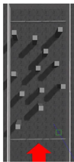
The server runs Ubuntu 16.04 with 3 NVIDIA TITAN Xp GPUs and the learning is implemented in Python 3.6 with Tensorflow 1.4 GPU. The trained models' weights and biases are transferred to the local machine running the simulation, and in addition to the accuracy evaluation of each model, real-time obstacle avoidance success rates will be compared. To determine the ability to avoid obstacles for each neural network, four additional test scenario maps were designed.
The obstacle layouts were randomized in such a way that patterns of the test cards were not provided during the training phase.
Training Results
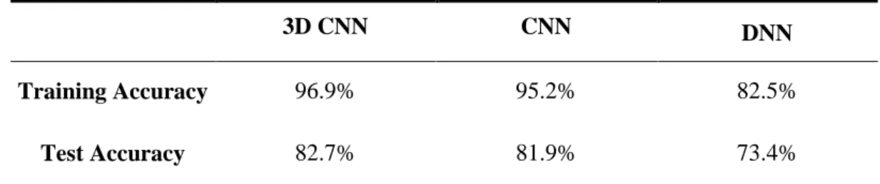
The accuracy of each network is calculated based on the number of correctly predicted values for a given number of samples. For each network, a total set of 500 randomly selected input batches from the test dataset were forwarded, with the 3D CNN showing the highest accuracy of the three, followed by the CNN and DNN. However, in terms of overall accuracy, the 3D CNN and CNN showed no significant difference.
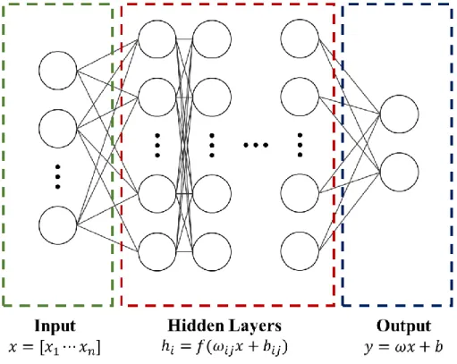
Based on the 3D CNN architecture discussed above, the confusion matrix is as shown below in Table 4. The results of the confusion matrix for each neural network were determined based on the 500 input bundles that were used to calculate the classification accuracy. The architecture of the DNN model used for comparison in this study is shown in Figure 16.
Three fully connected layers with 100 nodes each were used for DNN and the input was transformed into a 120*160 vector for the neural network.
Performance Evaluation Success Rate Evaluation
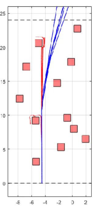
In addition to the overall success rates and individual trajectories for each trial, we analyzed the trajectories of the drones with respect to the distribution of the farthest points for each network in each map. Because the success rate only determines the success and failure of the test scenario in a Boolean way, we are able to more effectively analyze the performance of each network by visualizing the distribution of the farthest points, since the distance traveled at each trial reflects the obstacle avoidance of the network opportunities. The upper and lower edges of the box represent the upper and lower quartiles of the data distribution.
On maps 1, 2, and 3, CNN also showed that it was able to cover more than half of the map in most trials. However, the DNN was unable to successfully demonstrate obstacle avoidance ability as most of the furthest travel points were in the first half of the map. Based on the distributions obtained for each scenario, the average values of the maximum distance traveled for each case were compared.
The actual values are shown in Table 8, and the values are visualized in Figure 26 for comparison purposes. An additional metric to evaluate the performance of each neural network is to obtain an overall distribution of the points of the trajectory for each scenario. The bins used to obtain the point distribution are shown below in Figure 27.
From Figure 28, it can be noted that the 3D CNN and CNN both show consistent performances considering the point distribution of the trajectory points falling in each bin. Nevertheless, the trajectory point distribution of the CNN had some variations during the last quarter of the map. The DNN on the other hand, showed values of less than 0.4 for all the points outside the halfway point of the map, indicating that not many trajectory points are located further throughout the map.
The CNN showed a distribution of points with lower values near the end of the map, indicating that performance differences are present. We can conclude that the 3D CNN may have fluctuations in its performance under certain obstacle placement conditions. For the results for map 4 in Figure 31, since the 3D CNN was the only neural network that could avoid obstacles, the trajectory point distribution was 0 for most values near the end point in the case of CNN and DNN.
Although the 3D CNN only showed a 30% success rate for map 4, it can still be seen that the performance of the neural network was consistent.
CONCLUSION AND FUTURE WORK
1765-1772). IEEE