machine learning - based excited state molecular dynamics

(1)

저작자표시-비영리-변경금지 2.0 대한민국 이용자는 아래의 조건을 따르는 경우에 한하여 자유롭게

l 이 저작물을 복제, 배포, 전송, 전시, 공연 및 방송할 수 있습니다. 다음과 같은 조건을 따라야 합니다:

l 귀하는, 이 저작물의 재이용이나 배포의 경우, 이 저작물에 적용된 이용허락조건 을 명확하게 나타내어야 합니다.

저작권법에 따른 이용자의 권리는 위의 내용에 의하여 영향을 받지 않습니다. 이것은 이용허락규약(Legal Code)을 이해하기 쉽게 요약한 것입니다.

Disclaimer

저작자표시. 귀하는 원저작자를 표시하여야 합니다.

비영리. 귀하는 이 저작물을 영리 목적으로 이용할 수 없습니다.

변경금지. 귀하는 이 저작물을 개작, 변형 또는 가공할 수 없습니다.

(2)

Master’s Thesis

MACHINE LEARNING - BASED EXCITED STATE MOLECULAR DYNAMICS

Kicheol Kim

Department of Chemistry

Graduate School of UNIST

2019

(3)

MACHINE LEARNING - BASED EXCITED STATE MOLECULAR DYNAMICS

Kicheol Kim

Department of Chemistry

Graduate School of UNIST

(4)

(5)

(6)

Abstract

We present a new methodology for excited state molecular dynamics (ESMD) (or nonadiabatic molecular dynamics) based on machine learning (ML) technique. The most time consuming process in conventional on-the-fly ESMD simulations is an electronic structure calculation including analytic gradients of potential energy surfaces (PESs). Our study proposes that we can bypass this by exploiting ML.

We consider ensemble density functional theory, especially state-interaction state-averaged spin-restricted ensemble-referenced Kohn-Sham (SI-SA-REKS, or SSR for brevity) method as electronic structure calculation for the ML model since SSR(2,2) provides two diabatic electronic states, namely perfectly spin-paired singlet (PPS) and open-shell singlet (OSS), and their analytic gradients as well as interstate couplings (∆^SA).

In this study, we exploit the SchNetPack ML python library for ML procedure. For com- patibility, the decoherence-induced surface hopping based on exact factorization (DISH-XF) program is implemented in Python (pyDISH-XF) for nuclear dynamics. Some part of pyDISH- XF is written in C programming language to minimize the slowdown. We investigate ESMD of an ethylene molecule to benchmark pyDISH-XF. The performance of pyDISH-XF is better than UNI-xMD (a reference program is Fortran90). For overall ML-based ESMD, we focus on photo-induced cis-trans isomerization oftrans-Penta-2,4-dieniminium cation (PSB3), which is a typical model molecule for rhodopsin. The SchNet model is trained with 7500 and 50000 PSB3 geometries getting from previous ESMD studies. We get the poor result with 7500 training set, while the result with 50000 training set is reliable. Mean absolute error (MAE) energy and force of PPS is evaluated 0.01001 eV and 0.01750 eV/Å, MAE energy and force of OSS is evaluated 0.00888 eV and 0.01785 eV/Å, and MAE energy and force of∆^SA is evaluated 0.00948 eV and 0.03720 eV/Å.

We investigate ESMD of PSB3 with ML and compare the result with conventional ESMD of PSB3 with SSR method. The result is comparable to the conventional result. Furthermore, it takes 21 minutes using 1 cpu thread, while the conventional result takes 1.7 days using 2 gpu for propagating one trajectory.

(7)

(8)

List of Figures

1 Deep neural network structure. . . 2

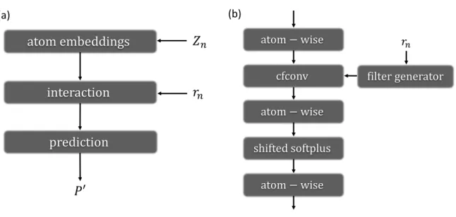
2 (a) Brief illustration of SchNet architecture. Zn is atomtype and rn is atomic coordinates each atomn. P⁰ is predicted property. (b) Illustration of interaction parts. . . 6

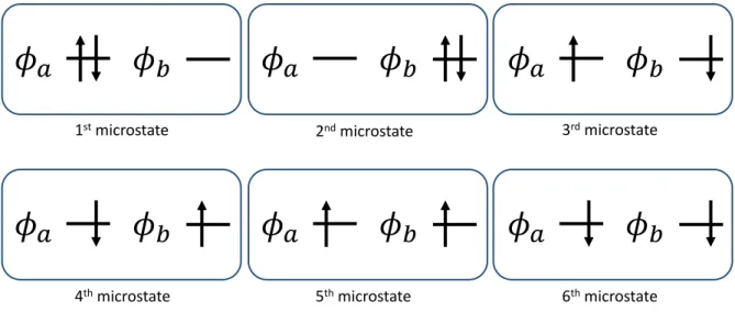
3 Six microstates in the SSR(2,2) method . . . 7

4 ML architecture to replace quantum mechanics . . . 19

5 FSSH dynamics of C₂H₄. . . 20

6 DISH-XF dynamics of C₂H₄. . . 21

7 (a) BO population of state 1 and state 2 at Surface Hopping. (b) BO population of state 1 and state 2 at DISH-XF . . . 21

8 (a) Difference of total energy, (b) difference of state 1 energy, (c) difference of state 2 energy at Surface Hopping. Corresponding to (d), (e), (f) at DISH-XF . . 22

9 (a) MAE energy of PPS, (b) MAE energy of OSS, (c) MAE energy of ∆^SA. (d) MAE force of PPS, (e) MAE force of OSS, (f) MAE force of ∆^SA . . . 24

10 BO populations of PSB3 ESMD . . . 25

11 BO populations of PSB3 ESMD with ML and SSR method . . . 26

(10)

List of Tables

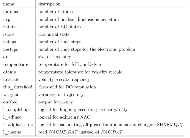
1 Input parameters of pyDISH-XF . . . 11 2 Setup for training model . . . 23 3 Evaluation result of the model . . . 25

(11)

Explanation of Terms and Abbreviations

ESMD BO MQC DFT ML DISH-XF

SI-SA-REKS, or SSR

eDFT PSB3 PPS OSS

pyDISH-XF FSSH ACSF DTNN cfconv CI FON KS MAE

Excited state molecular dynamics Born-Oppenheimer

Mixed quantum-classical Density functional theory Machine learning

Decoherence-induced surface hopping based on exact factorization State-interaction state-averaged spin-restricted ensemble- referenced Kohn-Sham

Ensemble DFT

Trans-Penta-2,4-dieniminium Cation Perfectly spin-paired singlet

Open-shell singlet

Python-based DISH-XF program Fewest switch surface hopping Atom-centered symmetry function Deep tensor neural network Continuous-filter convolutional Conical intersection

Fractional occupation number Kohn-Sham

Mean absolute error

(12)

I Introduction

Excited state molecular dynamics (ESMD) plays on the important role in photodynamic processes. Born-Oppenheimer (BO) approximation is known as a fundamental tool in chemical reactions. The BO approximation separates the motion of electrons and the motion of nuclei because electrons move much faster than nuclei. However, in ESMD, molecules pass through nonadiabatic coupling regions, where electron-nuclear correlation becomes strong, BO approximation fails to describe nonadiabatic behaviors between multiple BO electronic states. One of the most promising tools to describe the molecular dynamics in nonadiabatic coupling regions more precisely is mixed quantum-classical (MQC) method; nuclei obey classical dynamics while electrons obey quantum mechanics. One of the notable MQC methods is surface hopping technique that nuclei hop from one BO adiabatic surface to another BO adiabatic surface, if calculated hopping probability between two states satisfies some condition. Although many variants of surface hopping were introduced, most of them fails to describe quantum decoherence.

Another problem of existing ab initio-based molecular dynamics simulations is a short time scale. From ab initio to semi-empirical quantum chemistry methods, the quantum mechanical methods have struggled getting efficiency and accuracy. Hartree-Fock approximation is fundamental ab initio method. A many-body electronic wave function is expanded in terms of electronic orbitals,|Φ₀i=|φ₁φ₂...φ_ni. Fock operator is defined, fˆ= ˆh(1) +PN/2

j=1(2 ˆJ_j(1)−Kˆ_j(1)), whereˆh(1) =−¹₂∇²₁−P

I Z_I

r1I is one electron hamiltonian,Jˆ_j(1) =R

dr₂φ^∗_j(2)_r¹

12φ_j(2)is coulomb operator, andKˆj =R

dr2φ^∗_j(2)_r¹

12φi(2)is exchange operator. Then, solving eigenfunction equation,f φˆ _i =_iφ_i. The orbital energy of the electronic orbitalφ_i is _i. The Hartree-Fock method has defect neglected electron correlation. For considering electron correlation energy, configu- ration interaction, Møller-Plesset perturbation theory, and density functional theory (DFT) is suggested. However, time scale cannot exceed femtosecond which is very short time to describe realistic molecular dynamics. Machine learning (ML) is a rising methodology overcoming time scale problems.

ML is a task of creating a model that learns from arbitrary data and predicts uneducated values. In the field of machine learning, various kinds of models exist; support vector machine, decision tree learning, and so on. Among them, a deep neural network is in the spotlight.

Artificial neural networks are systems that mimic a human brain. Artificial neural networks are networked with artificial neurons,y =f(P

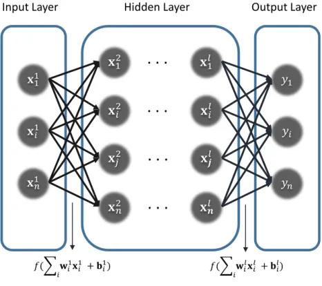
iw_ix_i+b_i), like that the neurons are connected by synapses to form the brain structures, where w is weights, x is features, b is bias, and f is activation function. Usually, nonlinear function (ex. sigmoid function) is used by activation function for making network more complicated. Deep neural network is neural network which has hidden layers between an input layer and an output layer as shown in Fig. 1. Layer is a group of artificial neurons. Supervised ML trains the model from a set of examples and labels, where an example is an instance of a feature, a label is a thing to be predicted. During training the model, a loss function is defined. A square error, l = (y−y⁰)², is commonly used for a

1

(13)

𝐱𝐱₁¹ 𝐱𝐱_𝑖𝑖¹ 𝐱𝐱_𝑛𝑛¹ Input Layer

𝑦𝑦₁ 𝑦𝑦_𝑖𝑖 𝑦𝑦_𝑛𝑛 Output Layer

𝐱𝐱

₁²

𝐱𝐱

_𝑖𝑖²

𝐱𝐱

_𝑗𝑗²

𝐱𝐱

𝑛𝑛2

Hidden Layer

𝐱𝐱

₁^𝑙𝑙

𝐱𝐱

_𝑖𝑖^𝑙𝑙

𝐱𝐱

_𝒋𝒋^𝑙𝑙

𝐱𝐱

_𝒏𝒏^𝑙𝑙

∙ ∙ ∙

𝑓𝑓(�𝑖𝑖𝐰𝐰_𝑖𝑖¹𝐱𝐱_𝑖𝑖¹ +𝐛𝐛_𝑖𝑖¹) 𝑓𝑓(�

𝑖𝑖𝐰𝐰_𝑖𝑖^𝑙𝑙𝐱𝐱_𝑖𝑖^𝑙𝑙 +𝐛𝐛_𝑖𝑖^𝑙𝑙)

Figure 1: Deep neural network structure.

loss function, where y is a label, y⁰ is a prediction. Then, gradients of weights and losses are calculated, and weights are adjusted to negative gradients for decreasing loss. After iterating those processes until a loss function minimizes, training is done.

ML has strengths in situations where it is difficult to formalize algorithms, such as reading pictures and judging what they are. In this respect, ML can be applied to quantum mechanical computation. This is because the result of quantum mechanics can be obtained through machine learning even if the exact formula is not utilized. There are many attempts to solve quantum mechanics problem through ML in various ways, such as learning to solve the Schrodinger equation [1] and the nonadiabatic excited-state dynamics [2].

In this study, ML is used for computing electronic structures in MQC dynamics. In previous studies, a new MQC formalism is suggested, where the nuclear dynamics follows a decoherence- induced surface hopping based on exact factorization (DISH-XF), while electronic states are obtained from the state-interaction state-averaged spin-restricted ensemble-referenced Kohn- Sham (SI-SA-REKS, or SSR) method based on the ensemble DFT (eDFT) [3]. Then, they are applied to the ESMD of the trans-Penta-2,4-dieniminium Cation (PSB3). Instead of the direct (or on-the-fly) SSR electronic structure calculation, a ML model implemented in SchNet

2

(14)

architecture [4] can predict the ground and excited state energies as well as their gradients and nonadiabatic coupling vectors. The model consists of 3 independent models which predict each of perfectly spin-paired singlet (PPS), open-shell singlet (OSS), and interstate coupling parameter, ∆^SA, energy and its gradient from the same atomic structure. DISH-XF algorithm is implemented in python program (pyDISH-XF). For much faster computation, C language code is interfaced in pyDISH-XF. In sectionII, we explain DISH-XF formalism, SchNet architecture, and SI-SA-REKS methodology briefly. In sectionIII, details of pyDISH-XF, suggested SchNet models to predict electronic properties, and combination of both pyDISH-XF and the model are given. In section IV, we explain the result so far; The verification of pyDISH-XF, training the ML model and ESMD of PSB3 with machine learning. In sectionV, we describe the conclusion of ongoing study.

3

(15)

II Theoretical Background

2.1 DISH-XF formalism

Tully’s fewest switch surface hopping (FSSH) is the most popular trajectory-based MQC method because of its simplicity and practicality. [5] Because of its fewest switch algorithm, nuclei only hop in nonadiabatic coupling region. FSSH calculates trajectories by Newtonian equation of motion, M^d_dt²^R2 = −∇E, and propagates electronic wave function Φ(r, t) by the time-dependent Schrödinger equation for electrons,i~_∂t^∂Φ(r, t) = ˆHBOΦ(r, t). BO expansion of an electronic wave function for nuclear trajectory Ris given as,

HˆBOΦ(r, t;R(t)) =X

i

Ci(t)φi(r;R(t)), (1) where φ_i(r;R(t)) is the wave function of ith BO state. If density matrix ρ_ik = C_i^∗(t)C_k(t) is defined, the electronic equation of motion can be expressed by the density matrix,

d

dtρ_ik(t) = i

~

{E_i(t)−E_k(t)}ρ_ik(t)

−X

j

{σ_ij(t)ρ_jk(t)−ρ_ij(t)σ_jk(t)} (2) whereEi is theith state BO energy,σ_jk is a nonadiabatic coupling matrix element between the jth andkth BO electronic states. However, FSSH lacks of quantum decoherence. To overcome this problem, DISH-XF method is suggested. [6]

In DISH-XF method, an additional electron-nuclear coupling term from exact factorization of a full molecular wave function [7–9] is introduced,

Q_jk =X

ν

i~ M_ν

∇_ν|χ|

|χ| |_R(t)·(fν,j−f_ν,k), (3) whereM_ν is the mass of theνth nucleus, ^∇_|χ|^ν^|χ| is a nuclear quantum momentum, andf_ν,j is an electronic phase atjth BO electronic state. Then, the electronic equation of motion yields,

d

dtρ_ik(t) =i

~

{E_i(t)−E_k(t)}ρ_ik(t)

−X

j

{σ_ij(t)ρ_jk(t)−ρij(t)σ_jk(t)}

+X

j

{Q_ji(t) +Q_jk(t)}ρ_ij(t)ρ_jk(t).

(4)

The nuclear quantum momenta are calculated from a set of auxiliary nuclear trajectories ap- proximately. An auxiliary trajectory R_k(t⁰) is generated when ρ_kk(t⁰) exceeds a threshold at time t⁰ (i.e. a notable population at thekth state). Then, the nuclear quantum momentum is given as,

∇_ν|χ|

|χ| |_R(t)=− 1

2σ²{R_k(t)− hR_k(t)i} (5) 4

(16)

wherehR_k(t)i=P

lρllR_lk(t), with uniform variance σ. The approximate electronic phase term is evaluated by time integration of momentum change, f_ν,i = −Rt

M_ν_dt^d0R_k(t⁰)dt⁰. There is a strong point that more accurate results can be obtained with less resources based on existing results. The hopping probability from the ith BO state to the kth BO state at time step size

∆tis calculated,

Pi→k = 2Re[ρ_ik(t)σ_ik(t)]

ρii(t) ∆t. (6)

If hopping probability Pi→k has negative value, it is set to 0. Also, because of total energy conservation, the hopping is forbidden if thekth BO energy,Ek, is greater than the total energy.

After hopping is done, the nuclear velocities are rescaled to satisfy the energy conservation.

DISH-XF algorithm is proceeded following steps; Step 1: Get BO potential energies each states and nonadiabatic coupling matrix elements, Step 2: Propagate electron density with decoherence term, Step 3: Nuclear dynamics is proceeded by Newtonian equation of motion, Step 4: Calculate hopping probability and determine hopping or not and generate decoherence terms.

2.2 SchNet

To apply ML in chemistry, featuring molecules is a crucial part. There are many tri- als to describe molecules. One of successful neural network architectures is Behler-Parrinello network. [10] In this network, atom-centered symmetry functions (ACSFs) represent atomistic systems. [11] ACSFs have two terms; radial and angular parts. First, a radial symmetry function is a sum of gaussians,

G^r_i =

all

X

j6=i

e^α(R^ij^−R^s⁾²f_c(R_ij), (7) where Rs is a shifted center of gaussian parameters, and fc(Rij) is a cutoff function with the width parameter α. Second, an angular symmetry function

G^a_i = 2^1−β

all

X

j,k6=i

(1 +λcosθ_ijk)^β×e^−α(R²^ij^+R²^ik^+R²^jk⁾fc(Rij)fc(R_ik)fc(R_jk), (8) is the sum of cosine functions of anglesθ_ijk centered at theith atom with an angular resolution parameter β. The parameter λcan have values+1or −1 corresponding toθijk = 0^◦ and 180^◦, respectively, which make maxima of the cosine function. ACSFs have benefits (1) invariance with respect to translation and rotation of the system, (2) independence of atomic coordinate.

For reliable ACSFs, finding suitable parameters is an important task. Thus, most of time are consumed to find proper parameters.

Deep tensor neural network (DTNN) solves above problems providing atom embedding and interaction refinements. [12] SchNet is one of variants of DTNN. Atoms are described tensor x_i∈R^F, with features F. x_i is initialized depending on an atomtypeZi,x_i =a_Z_i, where a_Z_i is a random value to be optimized during the training process. Each feature tensor is propagated through atom-wise layers, x_i=Wx_i+b. Because the same atoms share weights W and biasb,

5

(17)

atom embeddings interaction

prediction

𝑍𝑍

_𝑛𝑛

𝑟𝑟

_𝑛𝑛

𝑃𝑃𝑃

atom−wise cfconv atom−wise shifted softplus

atom−wise

filter generator 𝑟𝑟𝑛𝑛

(a) (b)

Figure 2: (a) Brief illustration of SchNet architecture. Z_nis atomtype and r_n is atomic coordinates each atom n. P⁰ is predicted property. (b) Illustration of interaction parts.

SchNet can apply any atomistic systems irrespective of the number of atoms. The interaction part refines atom embeddings with pairwise interactions of surrounding atoms. SchNet use continuous-filter convolutional (cfconv) layers. cfconv layers are used to generalize discrete convolutional layers. It is helpful to consider atomic positions without atomic coordinates. In this model, cfconv layers,

x_i =

natoms

X

j=0

x_j◦W^f(r_j−r_i), (9) with W^f : R³ → R^F that maps the atomic coordinates to features F, generated by filter- generating neural network. The operation ◦ represents an element-wise multiplication. Inter- action part consists of 3 atom-wise layers, cfconv layer and activation functions. Each layer is located in between atom-wise layers as shown in Fig. 2(b). Shifted softplus, ssp(x) = ln(0.5e^x+ 0.5), is used for activation functions. Filter-generating network considers rotational invariance and periodic boundary conditions within neighbor atoms. Neighbor atoms are atoms in a cutoff range. Prediction of given propertyP is a sum of atom-wise layer outputs,

P =

natoms

X

i

x_i. (10)

Instead of predicting atomic forces directly, SchNet differentiates a predicted energy function with respect to atomic positions,

F_i⁰(Z1, ..., Zn,r₁, ...,r_n) =−∂E⁰

∂r_i(Z1, ..., Zn,r₁, ...,r_n). (11) For the sake of training the model, SchNet minimizes the loss function, l(P, P⁰) =kP −P⁰k². For the training both energies and forces of molecular dynamics trajectories, a combined loss

6

(18)

function is used,

l((E⁰, F₁⁰, ...F_n⁰),(E, F₁, ...F_n)) =ρkE−E⁰k²+ 1−ρ n_atoms

natoms

X

i

kF_i−(−∂E⁰

∂r_i )k², (12) with trade-off parameterρ. [13]

2.3 SI-SA-REKS Method

We exploit the SSR method based on eDFT as an electronic structure calculation. [14–19] While the conventional DFT and time dependent DFT fail to capture the correct topology of the PESs in the conical intersections (CIs) vicinity, the SSR method enables much accurate description of the vertical excitation energies with the S1/S0 CIs matching the results calculated from the multireference ab initio wave function methods. The SSR methodology employs ground state eDFT to describe multireference ground states of molecules and eDFT for ensembles of ground and excited state to obtain excitation energies from a variational time-independent formalism.

The concept of the fractional occupation numbers (FONs) of several frontier Kohn-Sham (KS) orbitals appears due to the use of ensemble representation of the density and the energy. Here, we use the active space including two electrons in two KS orbitals (i.e. SSR(2,2)) to deal with theπ/π^∗ transitions of PSB3.

𝜙𝜙 _𝑎𝑎 𝜙𝜙 _𝑏𝑏

1^stmicrostate

𝜙𝜙 _𝑎𝑎 𝜙𝜙 _𝑏𝑏

2^ndmicrostate

𝜙𝜙 _𝑎𝑎 𝜙𝜙 _𝑏𝑏

3^rdmicrostate

𝜙𝜙 _𝑎𝑎 𝜙𝜙 _𝑏𝑏

4^thmicrostate

𝜙𝜙 _𝑎𝑎 𝜙𝜙 _𝑏𝑏

5^thmicrostate

𝜙𝜙 _𝑎𝑎 𝜙𝜙 _𝑏𝑏

6^thmicrostate

Figure 3: Six microstates in the SSR(2,2) method

In the SSR(2,2) method, the energy of the multireference state is expanded in terms of six microstates with the fixed and integer occupations of the active orbitalsφ_a andφ_b as shown in Fig. 3. The energies of ground and excited states are obtained by minimizing an ensemble of the PPS and OSS states with respect to the KS orbitals and their FONs. The energies of PPS and OSS states,E^{P P S} and E^OSS, are expressed as an ensemble average over six microstates as

E^{P P S} =

6

X

L=1

C_L^{P P S}E_L (13)

7

(19)

E^OSS =

6

X

L=3

C_L^OSSE_L (14)

whereC₁^{P P S} = ⁿ₂â,C₂^{P P S} = ⁿ₂^b,C₃^{P P S} =C₄^{P P S} =−C₅^{P P S} =−C₆^{P P S} =−^f⁽ⁿ₂â^/2), and C₃ÔSS = C₄ÔSS =−2C₅ÔSS =−2C₆ÔSS = 1 withn_a andn_b is FONs of the active KS orbitals eachφ_a and φb and f(na/2) = (nanb)^1−1/2((nâⁿ^b^+δ)/(1+δ)) with δ = 0.4 subject to na+nb = 2. The equal weightings in the SA-REKS(2,2) energyE^SA=w₀E^{P P S}+w₁EÔSS are chosen. Minimizing the SA-REKS(2,2) energy leads to a single particle equation,

n_pFˆ_pφ_p =X

q

^SA_pq φ_q (15)

where the Fock operatorFˆp of the pth orbitalφp is given by Fˆ_p =X

L

C_L^SAn^L_pαFˆ_α^L+n^L_pβFˆ_β^L np

(16) where p ∈ core, a, b. Here, the average occupation number n_p = P

LC_L^SA(n^L_pα+n^L_pβ) with C_L^SA =w₀C_L^{P P S} +w₁C_L^OSS, and the Largrangian matrix elements^SA_pq are obtained. The Fock operator of each microstate L is calculated within spin-restricted DFT framework.

So far, the S₀ and S₁ states are assumed decoupled by symmetry. If there is no symmetry or the two states belong in the same irreducible representation, we do not need to consider the interaction between the states. However, the assumption that the two states in SA-REKS(2,2) are decoupled by symmetry is often not realistic, thus the inclusion of states interactions becomes important. The interstate coupling∆^SAis calculated using the converged SA-REKS(2,2) Lagrangian matrix elements ^SA_ab between the active orbitals φ_a andφ_b as

∆^SA = (√

n_a−√

n_b)^SA_ab . (17)

The SSR states are obtained by solving the following2×2secular equation E^{P P S} ∆^SA

∆^SA E^OSS

! a00 a01

a₁₀ a₁₁

!

= E₀^SSR 0 0 E^SSR₁

! a00 a01

a₁₀ a₁₁

!

(18) Therefore, the ground and the lowest excited state energies,E₀^SSR and E₁^SSR, are obtained as

E_I^SSR=a²_0IE^{P P S}+a²_1IE^OSS+ 2a_0Ia_1I∆^SA (19) whereI = 0and1. The derivation of analytic gradients forE^{P P S},E^OSS, and∆^SAcan be found elsewhere. [20] The gradients of the SSR(2,2) states∇E_I^SSR are obtained as

∇E_I^SSR =a²_0I∇E^{P P S}+a²_1I∇E^OSS+ 2a_0Ia_1I∇∆^SA (20) The nonadiabatic coupling vectors can be expanded in terms of the gradients of the SSR(2,2)

8

(20)

states∇E_I^SSR and of the interstate coupling∇∆^SA, H₀₁= 1

E₁^SSR−E₀^SSR

2(a₀₀a₀₁−a₁₀a₁₁) a²₀₀−a²₀₁−a²₁₀+a²₁₁G₀₁

−2(a₀₀a₀₁−a₁₀a₁₁)(a₀₀a₁₀−a₀₁a₁₁) a²₀₀−a²₀₁−a²₁₀+a²₁₁ h₀₁ + (a₀₀a₁₁+a₀₁a₁₀)h₀₁

(21)

whereG₀₁= ¹₂(∇E₀^SSR− ∇E₁^SSR),h₀₁=∇∆^SA.

9

(21)

III Computational Method

3.1 Python-based DISH-XF program (pyDISH-XF)

pyDISH-XF is an object-oriented program whose classes are organized into individual processes.

All processes are managed as objects, which is advantageous for a large number of tasks. For faster computation, electron dynamics parts is implemented in C language and interfaced in pyDISH-XF using cython library.

1 from atoms i m p o r t Atoms

2 from bo i m p o r t Bo

3 from dynamics i m p o r t Dynamics

4 from sh i m p o r t Sh

5 from s h x f i m p o r t S h x f

6 from t h e r m o s t a t i m p o r t ∗

7 i m p o r t j s o n

8

9 i f __name__ == "__main__":

10 w i t h open(" unixmd . j s o n ") a s f :

11 a r g s = j s o n . l o a d ( f )

12 t r a j = Atoms (" unixmd . xyz ", a r g s )

13 bo = Bo ( a r g s )

14 sh = Sh ( a r g s )

15 s h x f = S h x f ( a r g s )

16 i f( a r g s [" thermo_type "] == " r e s c a l e 1 ") :

17 t h e r m o s t a t = v e l o c i t y _ r e s c a l e ( a r g s )

18 e l i f( a r g s [" thermo_type "] == " r e s c a l e 2 ") :

19 t h e r m o s t a t = v e l o c i t y _ r e s c a l e _ d t e m p ( a r g s )

20 e l s e:

21 t h e r m o s t a t = thermo ( a r g s )

22 md = Dynamics ( a r g s )

23 md . run ( t r a j , bo , sh , s h x f , t h e r m o s t a t )

The above code is a code example using pyDISH-XF. The parameters to define computations such as molecular dynamics scheme, thermostats, and initial conditions are received in a dictionary in the program or can be pre-declared externally through json. The types of input parameters are described in the table 1 below. After loading input parameters, getting input geometry from "unixmd.xyz" using Atoms class. Then, declare Bo, Sh, Shxf, thermostat and Dynamics objects. Bo object executes quantum mechanics program and parses energies, forces, and nonadiabatic coupling vector or matrix elements. Sh object calculates hopping probability and decides that hopping is occurred or not. Shxf object generates auxiliary trajectory and calculates decoherence terms. Finally, running molecular dynamics based on declared objects in Dynamics object.

10

(22)

name description natoms number of atoms

nsp number of nuclear dimensions per atom nstates number of BO states

istate the initial state nsteps number of time steps

nesteps number of time steps for the electronic problem

dt size of time step

temperature temperature for MD, in Kelvin

dtemp temperature tolerance for velocity rescale nrescale velocity rescale frequency

rho_threshold threshold for BO population wsigma variance for trajectory outfreq output frequency

l_simplehop logical for hopping according to energy only l_adjnac logical for adjusting NAC

l_allphase_dp logical for calculating all phase from momentum changes (SHXFMQC) l_nacme readNACME.DAT instead of NAC.DAT

Table 1: Input parameters of pyDISH-XF

3.1.1 API Document atoms.py

classAtoms(fname, args)

Get input geometry from given files.

Parameters: • fname(str) - name of input geometry file

• args(dictionary) - input parameters write_traj(dir)

Write current positions in TRAJECOTRY file.

Parameters: • dir(str) - path of proceeding calculation write_traj_xyz(dir)

Write current positions in TRAJECOTRY.xyz file in the .xyz format.

Parameters: • dir(str) - path of proceeding calculation write_movie(dir, first)

Accumulate current positions and velocities in MOVIE file as dynamics progresses.

11

(23)

Parameters: • dir(str) - path of proceeding calculation

• first(bool) - If true, write new MOVIE file.

write_movie_xyz(dir, first)

Accumulate current positions in MOVIE.xyz file in the .xyz format as dynamics progresses.

• first(bool) - If true, write new MOVIE.xyz file.

write_vel(dir)

Write current velocities in VELOCITY file.

Parameters: • dir(str) - path of proceeding calculation bo.py

classBo(args)

Class for quantum mechanics part of the system.

Parameters: • args(dictionary) - input parameters get_BO(dir, l_nac)

Run quantum mechanics program and call read_BO_files().

• l_nac(bool) - If true, calladjust_nac().

get_nacme(traj)

Get nonadiabatic coupling matrix elements from nonadiabatic coupling vectors.

Parameters: •traj(Atoms) -Atomsobject which has current atomic information.

adjust_nac()

Change sign of nonadiabatic coupling vectors if the overlap of current nonadiabatic coupling vectors and past nonadiabatic coupling vectors have negative sign.

read_BO_files()

Read energies, forces, and nonadiabatic coupling vectors or matrix elements which are got from quantum mechanics.

cl_dynamics.py classCl_dynamics(args)

Set classic mechanics part of the system.

Parameters: • args(dictionary) - input parameters cl_update_position(coef, traj, bo, sh)

Proceed to classical dynamics to obtain positions.

12

(24)

Parameters: • coef(np.array) - coefficients of BO wave function.

• traj(Atoms) - Atoms object which has current atomic information.

• bo(Bo) - Bo object which has current quantum mechanics information.

•sh(Sh) -Sh object which has current surface hopping information.

cl_update_position(coef, traj, bo, sh)

Proceed to classical dynamics to obtain positions.

cl_update_velocity(coef, traj, bo, sh)

Proceed to classical dynamics to obtain velocities.

calculate_force(coef, traj, bo, sh) Calculate nuclei forces.

dynamics.py classDynamics(args)

Class for main dynamics.

Parameters: • args(dictionary) - input parameters run(traj, bo, sh, shxf, thermostat)

Run MQC dynamics loop.

13

(25)

• shxf(Shxf) - Shxf object which has decoherence information.

• thermostat(thermo) - thermo object which has thermostat information.

write_md_trajinfo(traj)

Call write_traj() andwrite_traj_xyz()

write_md_output(istep, traj, bo, sh)

Callwrite_vel(),write_movie(),write_movie_xyz(),write_md_energy(),write_BO_coefs().

Iffirst is true, set first to false.

Parameters: • istep(int) - current dynamics step.

write_md_energy(istep, traj, bo, sh)

Accumulate kinetic energy, potential energy, and total energy in MDENERGY file.

Parameters: • istep(int) - current dynamics step.

write_BO_coefs()

Accumulate BO coefficient using density matrix diagonal term and off-diagonal term inBO- COEF file.

el_dynamics.pyx

el_propagator(el_propagator, nst, nat, nsp, nesteps, dt, wsigma, traj, bo, sh, shxf, rho, coef) Change python variables which using electron dynamics to C variable. Call C function for electron dynamics. Runge-Kutta method is used for propagating electron dynamics.

14

(26)

Parameters: • el_propagator(str) - method of electron propagator {coefficient or density}

• nst(int) - total number of states.

• nat(int) - total number of atoms.

• nsp(int) - total number of nuclear dimensions per atom.

• nesteps(int) - total number of time steps for electronic problem.

• dt(int) - size of time step.

• wsigma(int) - variance for trajectory.

• coef(np.array) - coefficients of BO wave function.

• rho(np.array) - coefficients density matrix of BO wave function.

sh.py classSh(args)

Class for surface hopping methods.

Parameters: • args(dictionary) - input parameters surface_hopping(dir, traj, bo, rho, istep)

Run surface hopping dynamics.

• istep(int) - current dynamics step.

hop_prob(rho, bo)

Calculate hopping probability.

Parameters: • rho(np.array) - coefficients density matrix of BO wave function.

write_sh_output(dir, rho)

Callwrite_sh_hopping_prob(),write_sh_running_state(), andwrite_sh_nacme(). Ifio_first is true, set io_first to false.

15

(27)

write_sh_nacme(dir, rho)

Write nonadiabatic coupling matrix elements in NACME file.

write_sh_hopping_prob(dir)

Accumulate hopping probability in SHPROB file.

Parameters: • dir(str) - path of proceeding calculation write_sh_running_state(dir)

Accumulate running state in SHSTATE file.

Parameters: • dir(str) - path of proceeding calculation shxf.py

classShxf(args)

Class for decoherence term.

Parameters: • args(dictionary) - input parameters decoherence_shxf(traj, bo, sh, rho, coef)

Run decoherence term calculation.

Parameters: • traj(Atoms) - Atoms object which has current atomic information.

get_aux_pos(traj, sh) Generate auxiliary trajectories.

get_aux_vel(traj, sh, bo)

Calculate velocity of auxiliary trajectories.

16

(28)

Parameters: • traj(Atoms) - Atoms object which has current atomic information.

get_nabph(traj, sh) Calculate electronic phase.

get_qmcdot(traj, sh, coef, rho)

Calculate decoherence term using BO coefficient.

thermostat.py classthermo(args)

Class for thermostat base.

Parameters: • args(dictionary) - input parameters classvelocity_rescale(args)

Class for thermostat which rescales velocities at each target step.

Parameters: • args(dictionary) - input parameters run(traj, shxf)

Rescale velocity at each target step.

classvelocity_rescale_dtemp(args)

Class for thermostat which rescales velocities if current temperature over temperature tolerance.

Parameters: • args(dictionary) - input parameters run(traj, shxf)

Rescale velocity if current temperature over temperature tolerance.

17

(29)

3.2 Extension of SchNet to excited states

Obtaining the ground and excited state energies, forces and nonadiabatic coupling vector is an object of quantum chemical calculations in DISH-XF. To replace quantum chemical calculations with ML, we have two choices in training processes; (1) training adiabatic properties, and (2) training diabatic properties. Since adiabatic electronic energies and their gradients can have nonanalytic behaviors in the vicinity of CIs, training diabatic energies and gradients may be more suitable choice for ESMD simulation. In this sense, SSR approach is beneficial since SSR provides diabatic states (PPS and OSS) and couplings (∆^SA) as well as gradients directly.

From identical atomic positions R_i, 3 independent SchNet models train each PPS, OSS, ∆^SA energy and force. Each model consists of F = 256 features and T = 6 interaction blocks. A cutoff radius is set to 20 Å, which can cover all atoms. Output layer is set predicting energy with force. For training the model, initial learning late is set to 0.0001. Instead of exponential decay, ReduceLRonPlateau method is used to decrease learning rate. It decreases learning late when training loss is not improved during the number of patience epoch. A combined loss function, l((E⁰, F₁⁰, ...F_n⁰),(E, F1, ...Fn)) =ρkE−E⁰k²+_n^1−ρ

atoms

Pnatoms

i kF_i−(−^∂E_∂r⁰

i)k², is used. All models are implemented based on SchNetPack. [4, 12, 21–25]

3.3 Combination of pyDISH-XF and SchNet

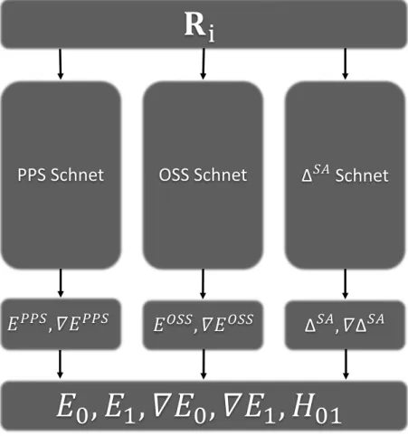
The SchNet models predict PPS, OSS, ∆^SA energies and forces. For the use in DISH-XF method, they should be converted into ground, excited energies and forces and nonadiabatic coupling vectors. Ground state energyE0, excited state energyE1, each of gradient∇E₀,∇E₁, and nonadiabatic coupling vector H₀₁ can be expressed as following equations. First, ground and excited energy can get from diagonalization of given matrix,

P⁻¹ E^{P P S} ∆^SA

∆^SA E^OSS

!

P = E₀ 0 0 E1

!

(22)

,where P is a00 a01

a₁₀ a₁₁

!

. Gradients of ground and excited state can be calculated the following equation,

∇E₀=a²₀₀∇E^{P P S} + 2a₀₀a₁₀∇∆^SA+a²₁₀∇E^OSS (23)

∇E₁=a²₀₁∇E^{P P S} + 2a11a01∇∆^SA+a²₁₁∇E^OSS. (24) Then, nonadiabatic coupling vector can be express as

H₀₁= 1 E1−E0

((a₀₀a₀₁−a₁₀a₁₁)g₀₁+ (a₀₀a₁₁+a₀₁a₁₀)h₀₁), (25) where g₀₁ = ¹₂(∇E^{P P S} − ∇E^OSS), and h₀₁ = ∇∆^SA. After getting energies, gradients, and nonadiabatic coupling vector, energies are written in ENERGY.DAT, forces Fi = −∇E_i are written in FORCE.DAT and nonadabatic coupling vector is written in NAC.DAT for parsing in pyDISH-XF program.

18

(30)

𝐑𝐑 _i

PPS Schnet OSS Schnet Δ

^{𝑆𝑆𝑆𝑆}

Schnet

𝐸𝐸

^{𝑃𝑃𝑃𝑃𝑆𝑆}

, 𝛻𝛻𝐸𝐸

^{𝑃𝑃𝑃𝑃𝑆𝑆}

𝐸𝐸

^{𝑂𝑂𝑆𝑆𝑆𝑆}

, 𝛻𝛻𝐸𝐸

^{𝑂𝑂𝑆𝑆𝑆𝑆}

Δ

^{𝑆𝑆𝑆𝑆}

, 𝛻𝛻 Δ

^{𝑆𝑆𝑆𝑆}

𝐸𝐸 ₀ , 𝐸𝐸 ₁ , 𝛻𝛻𝐸𝐸 ₀ , 𝛻𝛻𝐸𝐸 ₁ , 𝐻𝐻 ₀₁

Figure 4: ML architecture to replace quantum mechanics

19

(31)

IV Result and Discussion

4.1 Verification of pyDISH-XF program

To checking pyDISH-XF program, we perform ESMD of C₂H₄molecules. The initial geometry is set as a slightly modified the ground state geometry. We exploit DFTB/SSR method for electronic structure calculation. [26] Both FSSH and DISH-XF dynamics are done with UNI- xMD program [6] and pyDISH-XF program.

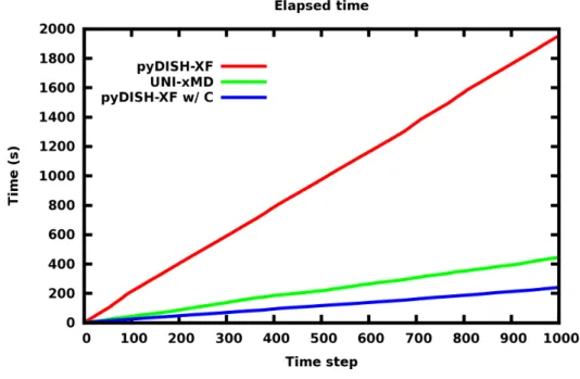
Figure 5: FSSH dynamics of C₂H₄.

FSSH dynamics is propagated up to 1000 steps with time step 0.12 fs shown in Fig. 5. Surface Hopping is done at 395th step forcibly for the same dynamics condition. UNI-xMD takes about 445 seconds. pyDISH-XF takes about 1952 seconds which is 4 times longer than UNI-xMD.

For finding the reason why it takes much time, time analysis is performed. Python has defect that is slowdown in loop state. We find that elapsed time is proportional to the number of loop steps. In electronic propagator, 10000 electronic steps is proceeded. As a result, the bottleneck is electronic propagator part of program. Alternatively using python, electronic propagator is altered C code. After that, pyDISH-XF interfaced with C code takes about 240 seconds which is 1.9 times faster than UNI-xMD program.

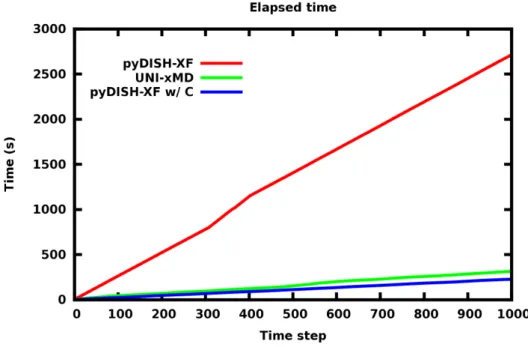
DISH-XF dynamics is also propagated up to 1000 steps with time step 0.12 fs shown in Fig. 6. Surface Hopping is done at 362th step forcibly for the same dynamics condition. UNI- xMD takes about 312 seconds. pyDISH-XF takes about 2711 seconds which is 8.6 times longer than UNI-xMD. Additional calculation of decoherence terms also takes long times in python.

It is not followed previous study that calculation of decoherence term is in the short time. [6]

After converting python to C code, it takes about 227 seconds which is 1.4 times faster than 20

(32)

Figure 6: DISH-XF dynamics of C₂H₄.

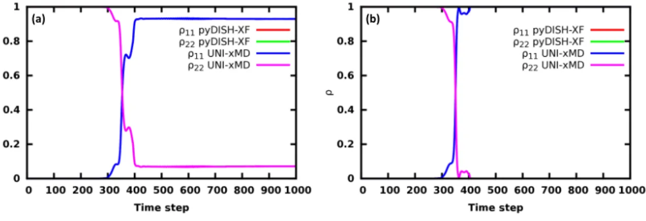
UNI-xMD program. Also, pyDISH-XF program obtains total energy, ground state energy and excited state energy within 1e-5 errors compared to UNI-xMD program both surface hopping and DISH-XF dynamics described in Fig. 8 and almost the same BO population of state 1 and state 2 obtained pyDISH-XF and UNI-xMD at the surface hopping and DISH-XF dynamics described in Fig. 7.

(a) (b)

Figure 7: (a) BO population of state 1 and state 2 at Surface Hopping. (b) BO population of state 1 and state 2 at DISH-XF

21

(33)

(a)(b)(c) (d)(e)(f) Figure8:(a)Differenceoftotalenergy,(b)differenceofstate1energy,(c)differenceofstate2energyatSurfaceHopping.Correspondingto (d),(e),(f)atDISH-XF

22

(34)

4.2 Training the model

Training dataset is calculated using the beta-testing version of the TeraChem program (v1.92P, release 7f19a3bb8334). [27–32] Total 62500 geometries are generated by ESMD of PSB3 that 50 trajectories are propagated up to 1250 steps with PPS and OSS of energies and gradients, and

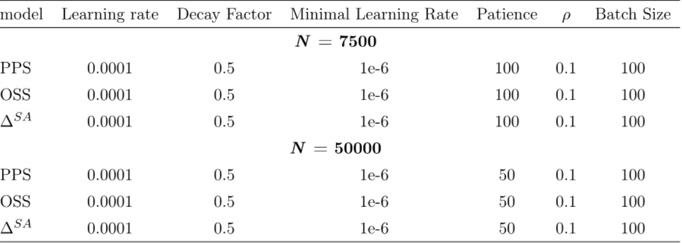
∆^SAand its gradients. We train the model with two different conditions which are summarized in Table 2. First, 7500 geometries by obtaining 1250 steps each 6 of trajectories are used to train the model with trade-off between energy force loss,ρ= 0.1and patience for ReduceLRonPlateau method is 100 at PPS, OSS and ∆^SA model. Initial learning rate is 1e-4. If the model is not improved during the number of patience epoch, learning rate is reduced to 0.5. Training is proceeded until learning rate is reduced to 1e-6. The model is trained with mini-batch stochastic gradient descent using ADAM optimizer. [33] Batch size is set to 100.

model Learning rate Decay Factor Minimal Learning Rate Patience ρ Batch Size N = 7500

PPS 0.0001 0.5 1e-6 100 0.1 100

OSS 0.0001 0.5 1e-6 100 0.1 100

∆^SA 0.0001 0.5 1e-6 100 0.1 100

N = 50000

PPS 0.0001 0.5 1e-6 50 0.1 100

OSS 0.0001 0.5 1e-6 50 0.1 100

∆^SA 0.0001 0.5 1e-6 50 0.1 100

Table 2: Setup for training model

Fig. 9 demonstrates the variation of mean absolute error (MAE) energy and force in PPS, OSS and ∆^SA model during training. MAE energies are more fluctuating than MAE forces, becauseρis set to give weight to force loss. Because∆^SAproperties are 1000 times smaller than PPS and OSS, ∆^SA model is converged much faster than PPS and OSS model.

We evaluate the models using 55,000 geometries by obtaining 1250 steps each 44 trajectories.

MAE energy and force of PPS are 0.32320 eV and 0.38730 eV/Å. MAE energy and force of OSS are 0.41073 eV and 0.44411 eV/Å. MAE energy and force of ∆^SA are 0.08501 eV and 0.20221 eV/Å. Compared to result of training set, all of MAEs are relatively high values. The result shows that this model predicts suitable properties only in training sets. It cannot be substituted SSR methods.

Then, we increase the training set from 7500 to 50000. It is randomly chosen from 62500 geometries by obtaining 1250 steps each 50 of trajectories. Patience for ReduceLRonPlateau method is 50 at PPS, OSS and ∆^SA model. MAE energy and force of PPS are reduced to 0.01001 eV and 0.01750 eV/Å. MAE energy and force of OSS are reduced to 0.00888 eV and 0.01785 eV/Å. MAE energy and force of∆^SAare reduced to 0.00948 eV and 0.03720 eV/Å. The

23

(35)

(a)(b)(c) (d)(e)(f) Figure9:(a)MAEenergyofPPS,(b)MAEenergyofOSS,(c)MAEenergyof∆SA .(d)MAEforceofPPS,(e)MAEforceofOSS,(f)MAE forceof∆SA

24

(36)

N = 7500 N = 50000

model MAE Energy (eV) MAE Force (eV/Å) MAE Energy (eV) MAE Force (eV/Å)

PPS 0.32320 0.38730 0.01001 0.01750

OSS 0.41073 0.44411 0.00888 0.01785

∆^SA 0.08501 0.20221 0.00948 0.03720

Table 3: Evaluation result of the model

results are summarized in Table 3. It is more suitable than the result getting from 7500 training model.

4.3 ESMD of PSB3 with Machine Learning

Total 100 trajectories are propagated up to 1250 steps with the time step 0.24 fs. Initial geometries are generated by the TeraChem software by Wigner sampling at T = 300 K in previous study. [3] We exploit pyDISH-XF with the SchNet model that is trained by 50000 training set.

Dynamics is proceeded under microcanonical ensemble.

Figure 10: BO populations of PSB3 ESMD

We analyze BO populations of PSB3 ESMD. Two types of BO populations are used; P_I is obtained from the numbers of trajectories running on the Ith state, hρ_IIi is averaged BO population over all trajectories. Out of 2 trajectories are not hopped that is the reason why final BO populations are not 0 and 1. Fig. 10 shows two types of BO populations have the same tendency that decoherence is well applied in ESMD.

We compare our result with ESMD of PSB3 with SSR method. [3] Both P_I and hρ_IIi have 25

(37)

Figure 11: BO populations of PSB3 ESMD with ML and SSR method

comparable result. DISH-XF with SSR dynamics takes 1.7 days to finish one trajectory using 2 gpu. However, DISH-XF with ML dynamics takes 21 minutes to finish one trajectory using 1 cpu thread. It gets 117 times faster result despite low computational cost.

26

(38)

V Conclusion

In this study, machine learning has been attempted to replace SSR methodology in DISH-XF formalism. pyDISH-XF is implemented with python interfaced with the external C code that propagates electronic steps for combining DISH-XF method and machine learning method easily.

ESMD of an ethylene molecule is proceeded with UNI-xMD program to benchmark pyDISH- XF program. pyDISH-XF program generates encouraging results that calculation is faster than UNI-xMD with reliable results.

The SchNet is used for training PPS, OSS and ∆^SA energies and forces. The model consists of three SchNet models each train three properties respectively implemented in SchNetPack;

deep neural network python library. PSB3 database is generated by the beta-testing version of the TeraChem program (v1.92P, release 7f19a3bb8334) which contains 62500 geometries consist of 1250 steps each 50 trajectories. However, the model trained with 7500 geometries couldn’t predict given properties; PPS, OSS, and ∆^SA energies and forces. Then, we increase training set from 7500 to 50000. As a result, the error is reduced then we proceed dynamics to using this model.

For comparing the result to conventional result, ESMD with machine learning is propagated in the same condition. It gets a comparable result within 21 minutes using 1 cpu thread compared to 1.7 day using 2 gpu at the conventional result. Therefore, we achieve the object that decreasing computational time.

27

(39)

References

[1] K. Mills, M. Spanner, and I. Tamblyn, “Deep Learning and the Schrödinger equation,”

Phys. Rev. A, vol. 96, p. 042113, 2017.

[2] W.-K. Chen, X.-Y. Liu, W.-H. Fang, P. O. Dral, and G. Cui, “Deep Learning for Nonadia- batic Excited-State Dynamics,” J. Phys. Chem. Lett., vol. 9, pp. 6702–6708, 2018.

[3] M. Filatov, S. K. Min, and K. S. Kim, “Direct Nonadiabatic Dynamics by Mixed Quantum- Classical Formalism Connected with Ensemble Density Functional Theory Method: Ap- plication to trans-Penta-2,4-dieniminium Cation,” J. Chem. Theory Comput., vol. 14, pp. 4499–4512, 2018.

[4] K. T. Schütt, H. E. Sauceda, P.-J. Kindermans, A. Tkatchenko, and K.-R. Müller, “SchNet - A deep learning architecture for molecules and materials,” J. Chem. Phys., vol. 148, p. 241722, 2018.

[5] J. C. Tully, “Molecular dynamics with electronic transitions,” J. Chem. Phys., vol. 93, p. 1061, 1990.

[6] J.-K. Ha, I. S. Lee, and S. K. Min, “Surface Hopping Dynamcis beyond Nonadiabatic Couplings for Quantum Coherence,” J. Phys. Chem. Lett., vol. 9, pp. 1097–1104, 2018.

[7] A. Abedi, N. T. Maitra, and E. K. U. Gross, “Exact Factorization of the Time-Dependent Electron-Nuclear Wave Function,” Phys. Rev. Lett., vol. 105, p. 123002, 2010.

[8] A. Abedi, N. T. Maitra, and E. K. U. Gross, “Correlated electron-nuclear dynamics: Exact factorization of the molecular wavefunction,” J. Chem. Phys., vol. 137, p. 22A530, 2012.

[9] N. I. Gidopoulos and E. K. U. Gross, “Electronic non-adiabatic states: towards a density functional theory beyond the Born–Oppenheimer approximation,” Philos. Trans. R. Soc.

A, vol. 372, p. 20130059, 2014.

[10] J. Behler and M. Parrinello, “Generalized Neural-Netwrok Representation of High- Dimensional Potential-Energy Surfaces,” Phys. Rev. Lett., vol. 98, p. 146401, 2007.

[11] J. Behler, “Atom-centered symmetry functions for constructing high-dimensional neural network potentials,” J. Chem. Phys., vol. 134, p. 074106, 2011.

28

(40)

[12] K. T. Schütt, F. Arbabzadah, S. Chmiela, K. R. Müller, and A. Tkatchenko, “Quantum- chemical insights from deep tensor neural networks,” Nat. Commun., vol. 8, p. 13890, 2017.

[13] A. Pukrittayakamee, M. Malshe, M. Hagan, L. M. Raff, R. Narulkar, S. Bukkapatnum, and R. Komanduri, “Simultaneous fitting of a potential-energy surface and its corresponding force fields using feedforward neural networks,” J. Chem. Phys., vol. 130, p. 134101, 2009.

[14] S. M. Valone, “A one-to-one mapping between one-particle densities and some n-particle ensembles,” J. Chem. Phys., vol. 73, p. 4653, 1980.

[15] E. H. Lieb, “Density functionals for coulomb systemses,” Int. J. Quantum Chem., vol. 24, pp. 243–277, 1983.

[16] J. P. Perdew, R. G. Parr, M. Levy, and J. Jose L. Balduz, “Density-Functional Theory for Fractional Particle Number: Derivative Discontinuities of the Energy,” Phys. Rev. Lett., vol. 49, pp. 1691–1694, 1982.

[17] H. Englisch and R. Englisch, “Hohenberg-Kohn theorem and non-V-representable densities,”

Phys. A, vol. 121, pp. 253–268, 1983.

[18] H. Englisch and R. Englisch, “Exact Density Functionals for Ground-State Energies. I.

General Results,” Phys. Status Solidi B, vol. 123, pp. 711–721, 1984.

[19] H. Englisch and R. Englisch, “Exact Density Functionals for Ground-State Energies II.

Details and Remarks,” Phys. Status Solidi B, vol. 124, pp. 373–379, 1984.

[20] M. Filatov, F. Liu, and T. J. Martínez, “Analytical derivatives of the individual state energies in ensemble density functional theory method. I. General formalism,” J. Chem.

Phys., vol. 147, p. 034133, 2017.

[21] K. T. Schütt, P. Kessel, M. Gastegger, K. A. Nicoli, A. Tkatchenko, and K.-R. Müller,

“SchNetPack: A Deep Learning Toolbox For Atomistic Systems,” J. Chem. Theory Com- put., vol. 15, pp. 448–455, 2019.

[22] K. T. Schütt, P.-J. Kindermans, H. Sauceda, S. Chmiela, A. Tkatchenko, and K.-R. Müller,

“SchNet: A continuous-filter convolutional neural network for modeling quantum interactions,” Adv. Neural Inf. Process. Syst., pp. 991–1001, 2017.

[23] M. Gastegger, L. Schwiedrzik, M. Bittermann, F. Berzsenyi, and P. Marquetand,

“wACSF—Weighted atom-centered symmetry functions as descriptors in machine learning potentials,” J. Chem. Phys., vol. 148, p. 241709, 2018.

[24] J. Behler and M. Parrinello, “Generalized Neural-Network Representation of High- Dimensional Potential-Energy Surfaces,” Phys. Rev. Lett., vol. 98, p. 146401, 2007.

29

machine learning - based excited state molecular dynamics

Master’s Thesis

MACHINE LEARNING - BASED EXCITED STATE MOLECULAR DYNAMICS

Kicheol Kim

Department of Chemistry

Graduate School of UNIST

2019

MACHINE LEARNING - BASED EXCITED STATE MOLECULAR DYNAMICS

Kicheol Kim

Department of Chemistry

Graduate School of UNIST

Abstract

Contents

List of Figures

List of Tables

Explanation of Terms and Abbreviations

I Introduction

𝐱𝐱

𝐱𝐱

𝐱𝐱

𝐱𝐱

𝐱𝐱

𝐱𝐱

𝐱𝐱

𝐱𝐱

∙ ∙ ∙

∙ ∙ ∙

∙ ∙ ∙

∙ ∙ ∙

II Theoretical Background

atom embeddings interaction

prediction

𝑍𝑍

𝑟𝑟

𝑃𝑃𝑃

𝜙𝜙 𝑎𝑎 𝜙𝜙 𝑏𝑏

𝜙𝜙 𝑎𝑎 𝜙𝜙 𝑏𝑏

𝜙𝜙 𝑎𝑎 𝜙𝜙 𝑏𝑏

𝜙𝜙 𝑎𝑎 𝜙𝜙 𝑏𝑏

𝜙𝜙 𝑎𝑎 𝜙𝜙 𝑏𝑏

𝜙𝜙 𝑎𝑎 𝜙𝜙 𝑏𝑏

III Computational Method

𝐑𝐑 i

PPS Schnet OSS Schnet Δ

Schnet

𝐸𝐸

, 𝛻𝛻𝐸𝐸

𝐸𝐸

, 𝛻𝛻𝐸𝐸

Δ

, 𝛻𝛻 Δ

𝐸𝐸 0 , 𝐸𝐸 1 , 𝛻𝛻𝐸𝐸 0 , 𝛻𝛻𝐸𝐸 1 , 𝐻𝐻 01

IV Result and Discussion

V Conclusion

References

𝜙𝜙 _𝑎𝑎 𝜙𝜙 _𝑏𝑏

𝜙𝜙 _𝑎𝑎 𝜙𝜙 _𝑏𝑏

𝜙𝜙 _𝑎𝑎 𝜙𝜙 _𝑏𝑏

𝜙𝜙 _𝑎𝑎 𝜙𝜙 _𝑏𝑏

𝜙𝜙 _𝑎𝑎 𝜙𝜙 _𝑏𝑏

𝜙𝜙 _𝑎𝑎 𝜙𝜙 _𝑏𝑏

𝐑𝐑 _i

𝐸𝐸 ₀ , 𝐸𝐸 ₁ , 𝛻𝛻𝐸𝐸 ₀ , 𝛻𝛻𝐸𝐸 ₁ , 𝐻𝐻 ₀₁