저작자표시-비영리-변경금지 2.0 대한민국 이용자는 아래의 조건을 따르는 경우에 한하여 자유롭게
l 이 저작물을 복제, 배포, 전송, 전시, 공연 및 방송할 수 있습니다. 다음과 같은 조건을 따라야 합니다:
l 귀하는, 이 저작물의 재이용이나 배포의 경우, 이 저작물에 적용된 이용허락조건 을 명확하게 나타내어야 합니다.
l 저작권자로부터 별도의 허가를 받으면 이러한 조건들은 적용되지 않습니다.
저작권법에 따른 이용자의 권리는 위의 내용에 의하여 영향을 받지 않습니다. 이것은 이용허락규약(Legal Code)을 이해하기 쉽게 요약한 것입니다.
Disclaimer
저작자표시. 귀하는 원저작자를 표시하여야 합니다.
비영리. 귀하는 이 저작물을 영리 목적으로 이용할 수 없습니다.
변경금지. 귀하는 이 저작물을 개작, 변형 또는 가공할 수 없습니다.
석사학위논문 2019년 2월
해양지중 저장 중
누출된 이산화탄소의 다중규모 확산 시뮬레이션을 위한 기초적인 연구
조선대학교 대학원
선박해양공학과
정 대 성
[UCI]I804:24011-200000267343
해양지중 저장 중
누출된 이산화탄소의 다중규모 확산 시뮬레이션을 위한 기초적인 연구
A Fundamental Study for
Numerical Simulation of Multi-Scale Diffusion of CO
2Leaked from Sea Floor
2019년 2월 25일
조선대학교 대학원
선박해양공학과
정 대 성
해양지중 저장 중
누출된 이산화탄소의 다중 규모 확산 시뮬레이션을 위한 기초적인 연구
지도교수 정 세 민
이 논문을 공학 석사학위신청 논문으로 제출함
2018년 10월
조선대학교 대학원
선박해양공학과
정 대 성
정대성의 석사학위논문을 인준함
위원장 조선대학교 교 수 권 영 섭 ( 인 ) 위 원 조선대학교 교 수 주 성 민 ( 인 ) 위 원 조선대학교 교 수 정 세 민 ( 인 )
2018 년 11 월
조선대학교 대학원
Contents
ABSTRACT
XVI제 1 장 서론
1제 1 절 배경
1제2절 관련 연구
9제3절 연구 목적
10제 2 장 다중규모 해양수치모델
11제1절 MEC-CO
2모델
11제2절 지배방정식
121. 중규모 영역 : 정수압 (Hydrostatic) 모델
122. 근방역 : Full 3D Lagrangian-Eulerian 모델
14제 3 장 수치 시뮬레이션
16제1절 시뮬레이션 조건
161. 해석 영역
162. 격자계
17가 . 중규모 영역
17나. 근방역
183. 경계 조건
194. 계산 조건
21가. 온도, 염분, 해수 중 용해된 CO
2(DCO
2) 초기조건
21나 . CO
2누출량 , 누출 비율 및 누출 지점
22다. 해석 parameter
23제2절 요약
24제 4 장 수치 시뮬레이션 결과
26제1절 조위 비교
26제2절 근방역
31제3절 중규모 영역
39제 4 절 결과 요약
45제 5 장 결론
47참고문헌 48
부록
A.1 격자 수렴도 테스트 53
A.2 근방역에서의 해수중 용해된 CO2(DCO2) 변화량(ΔC) 58 A.3 근방역에서의 CO2 분압(pCO2) 변화량(ΔpCO2) 70 A.4 중규모 영역에서의 해수중 용해된 CO2(DCO2) 변화량(ΔC) 82 A.5 중규모 영역에서의 CO2 분압(pCO2) 변화량ΔpCO2) 94
Table Contents
Table 1 Major countries′ NDC(Nationally Determined Contribution) for Paris Agreement ··· 2
Table 2 Greenhouse gases & their contribution to global warming ··· 3
Table 3 Cases for grid dependency test ··· 17
Table 4 Number of grids and sizes(dz) in z direction for grid dependency tests ··· 17
Table 5 Tidal components for simulation ··· 19
Table 6 Cases of leakage & initial CO2 bubble ratio ··· 22
Table 7 Simulation parameters ··· 23
Figure Contents
Fig. 1 The average global temperature index from 1880 to ongoing prediction analysis ··· 1
Fig. 2 CCS projects worldwide ··· 4
Fig. 3 Overview of CO2 storage technologies ··· 5
Fig. 4 Schematic view of CO2 leakage ··· 6
Fig. 5 Phase diagram of CO2··· 7
Fig. 6 Behavior of CO2 bubble/droplet in sea water ··· 7
Fig. 7 Quantitative criteria for biological impacts by ΔpCO2··· 8
Fig. 8 Candidate sites for geological storage of CO2 under sea floor ··· 10
Fig. 9 Comparison between (a) satellite view and (b) topography data in top view ··· 16
Fig. 10 Selected grid system for meso-scale region (No. of grid in x, y, z direction: 80 × 80 × 68) (a) top ward, (b) perspective views ··· 18
Fig. 11 Computed domain of small-scale region in meso-scale region ··· 18
Fig. 12 Location of small-scale region in (a) meso-scale region and (b) small-scale region grid ··· 19
Fig. 13 Initial condition (temparature [T], salinity [S], dissolved CO2 [DCO2, C] and density [R]) ··· 21
Fig. 14 Leakage area in small-scale region ··· 22
Fig. 15 Locations of tidal level comparison ··· 26
Fig. 16 Comparison of tidal level at north boundary(No. 4) ··· 27
Fig. 17 Comparison of tidal level at south boundary(No. 2) ··· 27
Fig. 18 Comparison of tidal level at east boundary(No. 3) ··· 27
Fig. 19 Comparison of tidal level at southeast boundary(No. 13) ··· 27
Fig. 20 Comparison of tidal level at northeast boundary(No. 14) ··· 28
Fig. 21 Comparison of tidal level near land area 1(No. 5) ··· 28
Fig. 22 Comparison of tidal level near land area 2(No. 6) ··· 28
Fig. 23 Comparison of tidal level near land area 3(No. 7) ··· 28
Fig. 24 Comparison of tidal level in the central area of simulation domain(No. 1) ··· 29
Fig. 25 Comparison of tidal level in the central area of simulation domain(No. 10) ··· 29
Fig. 26 Comparison of tidal level in the central area of simulation domain(No. 11) ··· 29
Fig. 27 Comparison of tidal level in the central area of simulation domain(No. 12) ··· 29
Fig. 28 Comparison of tidal level at leakage point(No. 8) ··· 30
Fig. 29 Comparison of tidal level in the southwest area of simulation domain(No. 9) ··· 30
Fig. 30 Comparison contour maps of void rate including leakage point in xz-plane(y=
1,125m) after 30 days of CO2 leakage with the different leakage amount in small scale region ((left): 3,800ton/year, (right): 94,600ton/year) ··· 31 Fig. 31 Comparison contour maps of void rate including leakage point in yz-plane(x=
1,125m) after 30 days of CO2 leakage with the different leakage amount in small scale region ((left): 3,800ton/year, (right): 94,600ton/year) ··· 32 Fig. 32 Comparison contour maps of ΔDCO2 including leakage point after 30 days of CO2
leakage with the different leakage amount in small scale region((a) : xz-plane(y= 1,125m), (b) : yz-plane(x= 1,125m)) ··· 33 Fig. 33 Comparison contour maps of ΔpCO2 including leakage point after 30 days of CO2
leakage with the different leakage amount in small scale region((a) : xz-plane(y= 1,125m), (b) : yz-plane(x= 1,125m)) ··· 34 Fig. 34 Comparison contour maps of ΔDCO2 including leakage point in xz-plane(y=
1,125m) with the different CO2 bubble ratio in small-scale region after (a) 10, (b) 20 and (c) 30 days of CO2 leakage ··· 35 Fig. 35 Comparison contour maps of ΔDCO2 including leakage point in yz-plane(x=
1,125m) with the different CO2 bubble ratio in small-scale region after (a) 10, (b) 20 and (c) 30 days of CO2 leakage ··· 36 Fig. 36 Comparison contour maps of ΔpCO2 including leakage point in xz-plane(y=
1,125m) with the different CO2 bubble ratio in small-scale region after (a) 10, (b) 20 and (c) 30 days of CO2 leakage ··· 37 Fig. 37 Comparison contour maps of ΔpCO2 including leakage point in yz-plane(x=
1,125m) with the different CO2 bubble ratio in small-scale region after (a) 10, (b) 20 and (c) 30 days of CO2 leakage ··· 38 Fig. 38 Comparison contour maps of ΔDCO2 including leakage point after 30 days of CO2
leakage with the different leakage amount in meso-scale region((a) : xz-plane(y= 108,000m), (b) : yz-plane(x= 63,000m)) ··· 39 Fig. 39 Comparison contour maps of ΔpCO2 including leakage point after 30 days of CO2
leakage with the different leakage amount in meso-scale region((a) : xz-plane(y= 108,000m), (b) : yz-plane(x= 63,000m)) ··· 40 Fig. 40 Comparison contour maps of ΔDCO2 including leakage point in xz-plane(y=
108,000m) with the different CO2 bubble ratio in meso-scale region after (a) 10, (b) 20 and (c) 30 days of CO leakage ··· 41
Fig. 41 Comparison contour maps of ΔDCO2 including leakage point in yz-plane(x=
63,000m) with the different CO2 bubble ratio in meso-scale region after (a) 10, (b) 20 and (c) 30 days of CO2 leakage ··· 42 Fig. 42 Comparison contour maps of ΔpCO2 including leakage point in xz-plane(y=
108,000m) with the different CO2 bubble ratio in meso-scale region after (a) 10, (b) 20 and (c) 30 days of CO2 leakage ··· 43 Fig. 43 Comparison contour maps of ΔpCO2 including leakage point in yz-plane(x=
63,000m) with the different CO2 bubble ratio in meso-scale region after (a) 10, (b) 20 and (c) 30 days of CO2 leakage ··· 44
부록 그림 목차
Fig. A.1-1 Location of comparison point ··· 53
Fig. A.1-2 Comparison of tidal level at No.1 ··· 53
Fig. A.1-3 Comparison of tidal level at No.2 ··· 53
Fig. A.1-4 Comparison of tidal level at No.3 ··· 54
Fig. A.1-5 Comparison of tidal level at No.4 ··· 54
Fig. A.1-6 Comparison of tidal level at No.5 ··· 54
Fig. A.1-7 Comparison of tidal level at No.6 ··· 54
Fig. A.1-8 Comparison of tidal level at No.7 ··· 55
Fig. A.1-9 Comparison of tidal level at No.8 ··· 55
Fig. A.1-10 Comparison of tidal level at No.9 ··· 55
Fig. A.1-11 Comparison of tidal level at No.10 ··· 55
Fig. A.1-12 Comparison of tidal level at No.11 ··· 56
Fig. A.1-13 Comparison of tidal level at No.12 ··· 56
Fig. A.1-14 Comparison of tidal level at No.13 ··· 56
Fig. A.1-15 Comparison of tidal level at No.14 ··· 56
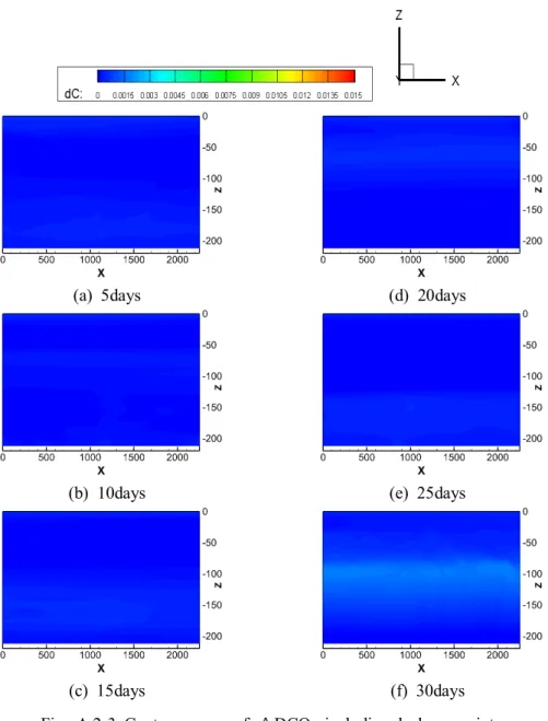
Fig. A.2-1 Contour maps of ΔDCO2 including leakage point in xz plane(y= 1,125m) in small-scale region after (a) 5, (b) 10, (c) 15, (d) 20, (e) 25 and (f) 30 days of CO2 leakage(case 1, 3,800ton/year, CO2 bubble ratio 10%) ··· 57
Fig. A.2-2 Contour maps of ΔDCO2 including leakage point in xz-plane(y= 1,125m) in small-scale region after (a) 5, (b) 10, (c) 15, (d) 20, (e) 25 and (f) 30 days of CO2 leakage(case 2, 3,800ton/year, CO2 bubble ratio 50%) ··· 58
Fig. A.2-3 Contour maps of ΔDCO2 including leakage point in xz-plane(y= 1,125m) in small-scale region after (a) 5, (b) 10, (c) 15, (d) 20, (e) 25 and (f) 30 days of CO2 leakage(case 3, 3,800ton/year, CO2 bubble ratio 90%) ··· 59
Fig. A.2-4 Contour maps of ΔDCO2 including leakage point in xz-plane(y= 1,125m) in small-scale region after (a) 5, (b) 10, (c) 15, (d) 20, (e) 25 and (f) 30 days of CO2 leakage(case 4, 94,600ton/year, CO2 bubble ratio 10%) ··· 60
Fig. A.2-5 Contour maps of ΔDCO2 including leakage point in xz-plane(y= 1,125m) in small-scale region after (a) 5, (b) 10, (c) 15, (d) 20, (e) 25 and (f) 30 days of CO2 leakage(case 5, 94,600ton/year, CO2 bubble ratio 50%) ··· 61
Fig. A.2-6 Contour maps of ΔDCO2 including leakage point in xz-plane(y= 1,125m) in small-scale region after (a) 5, (b) 10, (c) 15, (d) 20, (e) 25 and (f) 30 days of CO2
leakage(case 6, 94,600ton/year, CO2 bubble ratio 90%) ··· 62 Fig. A.2-7 Contour maps of ΔDCO2 including leakage point in yz-plane(x= 1,125m) in small-scale region after (a) 5, (b) 10, (c) 15, (d) 20, (e) 25 and (f) 30 days of CO2
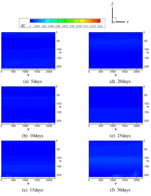
leakage(case 1, 3,800ton/year, CO2 bubble ratio 10%) ··· 63 Fig. A.2-8 Contour maps of ΔDCO2 including leakage point in yz-plane(x= 1,125m) in small-scale region after (a) 5, (b) 10, (c) 15, (d) 20, (e) 25 and (f) 30 days of CO2
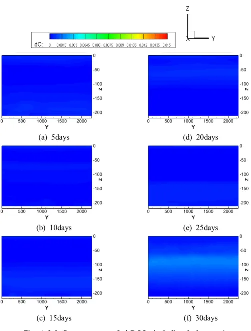
leakage(case 2, 3,800ton/year, CO2 bubble ratio 50%) ··· 64 Fig. A.2-9 Contour maps of ΔDCO2 including leakage point in yz-plane(x= 1,125m) in small-scale region after (a) 5, (b) 10, (c) 15, (d) 20, (e) 25 and (f) 30 days of CO2
leakage(case 3, 3,800ton/year, CO2 bubble ratio 90%) ··· 65 Fig. A.2-10 Contour maps of ΔDCO2 including leakage point in yz-plane(x= 1,125m) in small-scale region after (a) 5, (b) 10, (c) 15, (d) 20, (e) 25 and (f) 30 days of CO2
leakage(case 4, 94,600ton/year, CO2 bubble ratio 10%) ··· 66 Fig. A.2-11 Contour maps of ΔDCO2 including leakage point in yz-plane(x= 1,125m) in small-scale region after (a) 5, (b) 10, (c) 15, (d) 20, (e) 25 and (f) 30 days of CO2
leakage(case 5, 94,600ton/year, CO2 bubble ratio 50%) ··· 67 Fig. A.2-12 Contour maps of ΔDCO2 including leakage point in yz-plane(x= 1,125m) in small-scale region after (a) 5, (b) 10, (c) 15, (d) 20, (e) 25 and (f) 30 days of CO2
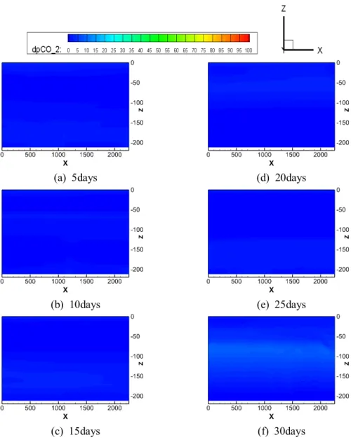
leakage(case 6, 94,600ton/year, CO2 bubble ratio 90%) ··· 68 Fig. A.3-1 Contour maps of ΔpCO2 including leakage point in xz-plane(y= 1,125m) in small-scale region after (a) 5, (b) 10, (c) 15, (d) 20, (e) 25 and (f) 30 days of CO2
leakage(case 1, 3,800ton/year, CO2 bubble ratio 10%) ··· 69 Fig. A.3-2 Contour maps of ΔpCO2 including leakage point in xz-plane(y= 1,125m) in small-scale region after (a) 5, (b) 10, (c) 15, (d) 20, (e) 25 and (f) 30 days of CO2
leakage(case 2, 3,800ton/year, CO2 bubble ratio 50%) ··· 70 Fig. A.3-3 Contour maps of ΔpCO2 including leakage point in xz-plane(y= 1,125m) in small-scale region after (a) 5, (b) 10, (c) 15, (d) 20, (e) 25 and (f) 30 days of CO2
leakage(case 3, 3,800ton/year, CO2 bubble ratio 90%) ··· 71 Fig. A.3-4 Contour maps of ΔpCO2 including leakage point in xz-plane(y= 1,125m) in small-scale region after (a) 5, (b) 10, (c) 15, (d) 20, (e) 25 and (f) 30 days of CO2
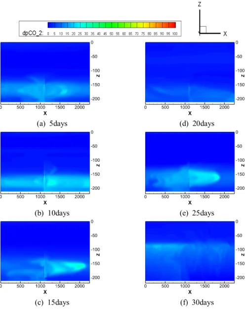
leakage(case 4, 94,600ton/year, CO2 bubble ratio 10%) ··· 72
Fig. A.3-5 Contour maps of ΔpCO2 including leakage point in xz-plane(y= 1,125m) in small-scale region after (a) 5, (b) 10, (c) 15, (d) 20, (e) 25 and (f) 30 days of CO2
leakage(case 5, 94,600ton/year, CO2 bubble ratio 50%) ··· 73 Fig. A.3-6 Contour maps of ΔpCO2 including leakage point in xz-plane(y= 1,125m) in small-scale region after (a) 5, (b) 10, (c) 15, (d) 20, (e) 25 and (f) 30 days of CO2
leakage(case 6, 94,600ton/year, CO2 bubble ratio 90%) ··· 74 Fig. A.3-7 Contour maps of ΔpCO2 including leakage point in yz-plane(x= 1,125m) in small-scale region after (a) 5, (b) 10, (c) 15, (d) 20, (e) 25 and (f) 30 days of CO2
leakage(case 1, 3,800ton/year, CO2 bubble ratio 10%) ··· 75 Fig. A.3-8 Contour maps of ΔpCO2 including leakage point in yz-plane(x= 1,125m) in small-scale region after (a) 5, (b) 10, (c) 15, (d) 20, (e) 25 and (f) 30 days of CO2
leakage(case 2, 3,800ton/year, CO2 bubble ratio 50%) ··· 76 Fig. A.3-9 Contour maps of ΔpCO2 including leakage point in yz-plane(x= 1,125m) in small-scale region after (a) 5, (b) 10, (c) 15, (d) 20, (e) 25 and (f) 30 days of CO2
leakage(case 3, 3,800ton/year, CO2 bubble ratio 90%) ··· 77 Fig. A.3-10 Contour maps of ΔpCO2 including leakage point in yz-plane(x= 1,125m) in small-scale region after (a) 5, (b) 10, (c) 15, (d) 20, (e) 25 and (f) 30 days of CO2
leakage(case 4, 94,600ton/year, CO2 bubble ratio 10%) ··· 78 Fig. A.3-11 Contour maps of ΔpCO2 including leakage point in yz-plane(x= 1,125m) in small-scale region after (a) 5, (b) 10, (c) 15, (d) 20, (e) 25 and (f) 30 days of CO2
leakage(case 5, 94,600ton/year, CO2 bubble ratio 50%) ··· 79 Fig. A.3-12 Contour maps of ΔpCO2 including leakage point in xz-plane(y= 1,125m) in small-scale region after (a) 5, (b) 10, (c) 15, (d) 20, (e) 25 and (f) 30 days of CO2
leakage(case 6, 94,600ton/year, CO2 bubble ratio 90%) ··· 80 Fig. A.4-1 Contour maps of ΔDCO2 including leakage point in xz-plane(y= 108,000m) in meso-scale region after (a) 5, (b) 10, (c) 15, (d) 20, (e) 25 and (f) 30 days of CO2
leakage(case 1, 3,800ton/year, CO2 bubble ratio 10%) ··· 81 Fig. A.4-2 Contour maps of ΔDCO2 including leakage point in xz-plane(y= 108,000m) in meso-scale region after (a) 5, (b) 10, (c) 15, (d) 20, (e) 25 and (f) 30 days of CO2
leakage(case 2, 3,800ton/year, CO2 bubble ratio 50%) ··· 82 Fig. A.4-3 Contour maps of ΔDCO2 including leakage point in xz-plane(y= 108,000m) in meso-scale region after (a) 5, (b) 10, (c) 15, (d) 20, (e) 25 and (f) 30 days of CO2
leakage(case 3, 3,800ton/year, CO2 bubble ratio 90%) ··· 83
Fig. A.4-4 Contour maps of ΔDCO2 including leakage point in xz-plane(y= 108,000m) in meso-scale region after (a) 5, (b) 10, (c) 15, (d) 20, (e) 25 and (f) 30 days of CO2
leakage(case 4, 94,600ton/year, CO2 bubble ratio 10%) ··· 84 Fig. A.4-5 Contour maps of ΔDCO2 including leakage point in xz-plane(y= 108,000m) in meso-scale region after (a) 5, (b) 10, (c) 15, (d) 20, (e) 25 and (f) 30 days of CO2
leakage(case 5, 94,600ton/year, CO2 bubble ratio 50%) ··· 85 Fig. A.4-6 Contour maps of ΔDCO2 including leakage point in xz-plane(y= 108,000m) in meso-scale region after (a) 5, (b) 10, (c) 15, (d) 20, (e) 25 and (f) 30 days of CO2
leakage(case 6, 94,600ton/year, CO2 bubble ratio 90%) ··· 86 Fig. A.4-7 Contour maps of ΔDCO2 including leakage point in yz-plane(x= 63,000m) in meso-scale region after (a) 5, (b) 10, (c) 15, (d) 20, (e) 25 and (f) 30 days of CO2
leakage(case 1, 3,800ton/year, CO2 bubble ratio 10%) ··· 87 Fig. A.4-8 Contour maps of ΔDCO2 including leakage point in yz-plane(x= 63,000m) in meso-scale region after (a) 5, (b) 10, (c) 15, (d) 20, (e) 25 and (f) 30 days of CO2
leakage(case 2, 3,800ton/year, CO2 bubble ratio 50%) ··· 88 Fig. A.4-9 Contour maps of ΔDCO2 including leakage point in yz-plane(x= 63,000m) in meso-scale region after (a) 5, (b) 10, (c) 15, (d) 20, (e) 25 and (f) 30 days of CO2
leakage(case 3, 3,800ton/year, CO2 bubble ratio 90%) ··· 89 Fig. A.4-10 Contour maps of ΔDCO2 including leakage point in yz-plane(x= 63,000m) in meso-scale region after (a) 5, (b) 10, (c) 15, (d) 20, (e) 25 and (f) 30 days of CO2
leakage(case 4, 94,600ton/year, CO2 bubble ratio 10%) ··· 90 Fig. A.4-11 Contour maps of ΔDCO2 including leakage point in yz-plane(x= 63,000m) in meso-scale region after (a) 5, (b) 10, (c) 15, (d) 20, (e) 25 and (f) 30 days of CO2
leakage(case 5, 94,600ton/year, CO2 bubble ratio 50%) ··· 91 Fig. A.4-12 Contour maps of ΔDCO2 including leakage point in yz-plane(x= 63,000m) in meso-scale region after (a) 5, (b) 10, (c) 15, (d) 20, (e) 25 and (f) 30 days of CO2
leakage(case 6, 94,600ton/year, CO2 bubble ratio 90%) ··· 92 Fig. A.5-1 Contour maps of ΔpCO2 including leakage point in xz-plane(y= 108,000m) in meso-scale region after (a) 5, (b) 10, (c) 15, (d) 20, (e) 25 and (f) 30 days of CO2
leakage(case 1, 3,800ton/year, CO2 bubble ratio 10%) ··· 93 Fig. A.5-2 Contour maps of ΔpCO2 including leakage point in xz-plane(y= 108,000m) in meso-scale region after (a) 5, (b) 10, (c) 15, (d) 20, (e) 25 and (f) 30 days of CO2
leakage(case 2, 3,800ton/year, CO2 bubble ratio 50%) ··· 94
Fig. A.5-3 Contour maps of ΔpCO2 including leakage point in xz-plane(y= 108,000m) in meso-scale region after (a) 5, (b) 10, (c) 15, (d) 20, (e) 25 and (f) 30 days of CO2
leakage(case 3, 3,800ton/year, CO2 bubble ratio 90%) ··· 95 Fig. A.5-4 Contour maps of ΔpCO2 including leakage point in xz-plane(y= 108,000m) in meso-scale region after (a) 5, (b) 10, (c) 15, (d) 20, (e) 25 and (f) 30 days of CO2
leakage(case 4, 94,600ton/year, CO2 bubble ratio 10%) ··· 96 Fig. A.5-5 Contour maps of ΔpCO2 including leakage point in xz-plane(y= 108,000m) in meso-scale region after (a) 5, (b) 10, (c) 15, (d) 20, (e) 25 and (f) 30 days of CO2
leakage(case 5, 94,600ton/year, CO2 bubble ratio 50%) ··· 97 Fig. A.5-6 Contour maps of ΔpCO2 including leakage point in xz-plane(y= 108,000m) in meso-scale region after (a) 5, (b) 10, (c) 15, (d) 20, (e) 25 and (f) 30 days of CO2
leakage(case 6, 94,600ton/year, CO2 bubble ratio 90%) ··· 98 Fig. A.5-7 Contour maps of ΔpCO2 including leakage point in yz-plane(x= 63,000m) in meso-scale region after (a) 5, (b) 10, (c) 15, (d) 20, (e) 25 and (f) 30 days of CO2
leakage(case 1, 3,800ton/year, CO2 bubble ratio 10%) ··· 99 Fig. A.5-8 Contour maps of ΔpCO2 including leakage point in yz-plane(x= 63,000m) in meso-scale region after (a) 5, (b) 10, (c) 15, (d) 20, (e) 25 and (f) 30 days of CO2
leakage(case 2, 3,800ton/year, CO2 bubble ratio 50%) ··· 100 Fig. A.5-9 Contour maps of ΔpCO2 including leakage point in yz-plane(x= 63,000m) in meso-scale region after (a) 5, (b) 10, (c) 15, (d) 20, (e) 25 and (f) 30 days of CO2
leakage(case 3, 3,800ton/year, CO2 bubble ratio 90%) ··· 101 Fig. A.5-10 Contour maps of ΔpCO2 including leakage point in yz-plane(x= 63,000m) in meso-scale region after (a) 5, (b) 10, (c) 15, (d) 20, (e) 25 and (f) 30 days of CO2
leakage(case 4, 94,600ton/year, CO2 bubble ratio 10%) ··· 102 Fig. A.5-11 Contour maps of ΔpCO2 including leakage point in yz-plane(x= 63,000m) in meso-scale region after (a) 5, (b) 10, (c) 15, (d) 20, (e) 25 and (f) 30 days of CO2
leakage(case 5, 94,600ton/year, CO2 bubble ratio 50%) ··· 103 Fig. A.5-12 Contour maps of ΔpCO2 including leakage point in yz-plane(x= 63,000m) in meso-scale region after (a) 5, (b) 10, (c) 15, (d) 20, (e) 25 and (f) 30 days of CO2
leakage(case 6, 94,600ton/year, CO2 bubble ratio 90%) ··· 104
ABSTRACT
A Fundamental Study for Numerical Simulation of Multi-Scale Diffusion of CO
2Leaked from Sea Floor
Jeong Dae Sung
Advisor : Prof. Jeong Se-Min, Ph.D.
Department of Naval Architecture & Ocean Engineering Graduate School of Chosun University
Carbon Capture and Storage(CCS) is a technology to capture and store carbon dioxide(CO2), which is a representative greenhouse gas. Since its potential to reduce large amount of CO2and feasibility, many countries are working on various CCS methods and projects. CCS can be categorized by geological sequestration(=storage), ocean sequestration and geological sequestration under seafloor, among which the last one is the most proper option to Korea since there is not enough inland space to store CO2. However, public acceptance is an unknown factor in developing public policy involving CCS technology.
Characteristics of CCS substantially differ from other options for CO2 mitigation, particularly when assessing the risks of leakage and development of appropriate regulatory penalties in implementing some form of CCS. Therefore, to carry out geological sequestration of CO2 under seafloor, it is inevitable to evaluate the risk of leakage, to monitor the behavior of leaked CO2and to assess the environmental effect by the leaked CO2.
The CO2 in seawater can exist as liquid or gas phase depending on its surrounding environments, mainly pressure and temperature. Therefore, the behavior of CO2 bubbles with dissolving into surrounding sea-water and diffusion of dissolved CO2
(DCO2) by ocean flows should be accurately predicted for the assessment of environmental impacts.
In this study, the behavior and diffusion of CO2, which is purposely stored under seafloor and leaked from it, bubbles and DCO2 in the sea-water was numerically predicted by multi-scale ocean model, where hydrostatic approximation and Eulerian-Lagragian two phase model is applied for meso- and small-scale region, respectively. Two cases are selected by assumed leaking-amount of CO2, that is 3,800ton/year and 94,600ton/year, and numerical simulations are performed for the cases. The results including the change of partial pressure of CO2(pCO2), which is one of the most important criteria for environmental impacts on marine biota, are qualitatively compared with each other.
제 1 장 서론
제1절 배경
1880년부터 최근까지 지구의 평균 온도가 지속적으로 증가하고 있으며, 2020 년 이후에도 증가할 것이라 예측된다(Fig. 1).
Fig. 1 The average global temperature index from 1880 to ongoing prediction analysis
<https://climate.nasa.gov/vital-signs/global-temperature/>
지구의 평균 온도 상승으로 발생하는 지구 온난화는 해양 및 대기의 온도를 상승시키며, 이로 인하여 해양환경에 영향을 미친다. 해양의 온도가 증가하면, 해 수면상승으로 인하여 저지대의 침수, 지하수위의 상승, 해안지역의 침식 및 퇴적 환경의 변화와 더불어 폭풍 영향권의 확대와 하천에서 해수의 침투거리가 길어 짐에 따라 생활용수의 취수 장애 등이 발생할 수 있으며, 해양생태계의 교란을 발생시킨다(석문식, 1991). 이중 열대 해양 생물 중 하나인 산호는 온도가 상승할 경우 서로 먹이를 공급하는 공생관계인 조류들이 산호의 주변을 이탈하는 백화 현상(Coral bleaching)이 발생하며, 이로 인하여 생존이 어려워진다. Lesser(1997)은 해양온도 상승이 산호의 백화현상에 영향을 미친다는 것을 실험을 통하여 결론 지었다.
또한 해양의 온도 상승은 해양의 산성화(pH값 감소)를 야기시킨다. Pörtner et
al.(2004)은 해양생물이 낮은 pH에 노출될 경우, 해양 생물의 신진대사율과 산소
공급율을 감소시키는 것을 분석하였으며, Kroeker et al.(2013)은 해양 산성화가 다양한 생물 군의 생존, 성장 등에 미치는 영향에 대해 실험하였으며, pH가 감소 할 경우, 생물 군의 생존, 성장 등이 감소하는 것을 실험하였다.
이러한 해양환경에 영향을 미치는 지구 온난화의 원인을 세계기상기구(World Meteorological Organization, WMO)와 국제연합환경계획(United Nations Environment Program, UNEP)은 산업 발전 등의 과도한 에너지 사용으로 발생하 는 온실가스의 증가로 규정했다.
세계적으로 온실가스의 배출을 줄이기 위해, 2015년 파리에서 열린 유엔 기 후 변화 회의(The United Nations Frameworks Convention on Climate, UNFCCC)를 통하여 파리협정(Paris Agreement)을 체결하였다. Table 1은 파리협정에서 각국이 자국 상황에 맞게 설정한 온실가스 감축목표(Nationally Determined Contribution,
NDC)를 보이고 있다. 이 중 대한민국은 2030년까지 온실가스 배출전망치
(Business as Usual, BAU)인 8억 5,060만 톤 대비 37% 감축을 목표로 하고 있다.
Object
Nation 감축목표 목표연도 기준연도 목표유형 국제탄소시장
사용여부
중국 60 ~ 65% 2030 2005 집약도 -
E.U. 40 % 2030 1990 절대량 X
러시아 25 ~ 30% 2030 1990 절대량 X
일본 26 % 2030 2013 절대량 O
대한민국 37 % 2030 - BAU O
Table 1 Major countries′ NDC(Nationally Determined Contribution) for Paris Agreement
<http://ebizdiary.tistory.com/513>
배출을 저감시켜야하는 온실가스의 종류는 이산화탄소(CO2), 메탄(CH4), 아산 화질소(N2O), 수소불화탄소(HFCS), 과불화탄소(PFCS), 육불화황(SF6)로 교토의정서
(Kyoto Protocol, 1997)에서 규정되었으며, 파리협정(2015)에서도 동일하게 규정하
였다. Table 2은 규정된 온실가스의 종류별 배출원과, 지구온난화지수, 온난화기
여도 및 국내 배출량을 나타낸다. 지구온난화지수는 온실가스 1kg의 태양에너지 를 흡수량이며, 온실가스 중 이산화탄소 1kg의 흡수량을 1로 설정한 값이다.
HFCS, PFCS, SF6는 CO2보다 지구온난화지수는 더 높지만, 온난화기여도와 국내 배출량을 고려하였을 때, 국내 배출량과 온난화기여도의 수치가 낮기 때문에, 지 구온난화에 CO2가 타 온실가스보다 더 많은 영향을 미친다고 할 수 있다.
GHG Type
CO2 CH4 N20 HFCS,
PFCS, SF6
배출원 에너지사용
/산업공정
폐기물/농업 /축산
산업공정
/비료사용
냉매
/세척용
지구온난화지수
(CO2 = 1) 1 21 310 1,300 ~
23,900 온난화기여도
(%) 55 15 6 24
국내 배출량
(%) 88.6 4.8 2.8 3.8
Table 2 Greenhouse gases & their contribution to global warming
<https://gscaltexmediahub.com/energy/about-greenhouse-gas/>
CO2를 저감시키는 기술에는 CO2 배출을 저감시키는 기술과 공기 중에 배출 된 CO2를 저감시키는 기술이 있다. CO2 배출을 저감시키는 방법은 화석연료의 사용을 줄이거나, 이를 대체할 신재생에너지를 개발, 사용하여 배출량을 줄이는 방법과 배출구에 Filter 등을 장비시켜 CO2의 배출을 줄이는 기술 등이 있다. 공 기 중에 배출된 CO2를 저감시키는 기술은 배출된 CO2를 포집하여 저장하는 기 술인 탄소 포집 및 저장(Carbon Captured and Storage, CCS) 기술과 포집 후 다른 물질로 변환하여 저장하는 탄소 포집 및 이용(Carbon Captured and Utilization,
CCU) 기술이 있다. 이중 CCS는 다른 저감 기술에 비하여 CO2를 대규모로 감축
가능한 장점이 있으며, 세계적으로 많은 Project가 수행되면서 안정적인 CO2 저감 기술로 알려져 있다. Fig. 2는 세계적으로 수행 중인 CCS Project를 보이고 있다.
Fig. 2 CCS projects worldwide
<https://pubs.rsc.org/en/content/articlehtml/2009/ee/b822107n>
CCS의 CO2를 저장(Storage/Sequestration)하는 방법은 Fig. 3와 같이 저장하는 공간의 위치로 분류된다. 육지에서 유전 및 천연가스 등의 자원을 채굴 후 발생 한 공간에 CO2를 저장하는 방법인 지중 저장(Geological Sequestration)법과 CO2를 해양에 저장 혹은 용해시키는 방법인 해양 저장(Ocean Sequestration)법이 있다. 해양 저장법은 해양에 액체상의 CO2를 용해시키는 방법인 용해법(Dissolution Type)과, 해양 지중에 저장하는 해양지중 저장법(Geological Sequestration under the
Seafloor) 등이 있다. 이중 해양 직접 용해법은 CO2가 해양환경에 미치는 영향의
불확실성으로 인하여 2007년 런던회의를 통하여 금지되었다.
Fig. 3 Overview of CO2 storage technologies
Kang & Huh(2008)은 다른 국가들의 CCS 연구 개발동향을 분석하여 국내 실
용화 방안에 대하여 분석하였다. 그 결과, 우리나라의 경우는 지중저장법을 실행 하기 위한 육상 공간이 부족하여 인근 해역에의 해양지중 저장법이 타당하다고 하였다.
해양지중 저장법을 통하여 CO2를 저장하기 위해서는 공적 수용성(Public
Acceptance) 확보가 필요하다. 이를 위해서는 지진 등의 재해 발생으로 저장 장소
에 균열이 발생하여 해양지중에 저장된 CO2가 해수로 누출되는 경우(Fig. 4), 누 출된 CO2가 주변 해양환경에 미치는 위험도 평가와 누출 지점에서 누출된 CO2
의 거동 모니터링 및 누출 후 해수로 용해된 CO2의 해수중 대류 및 확산에 대한 예측과 이에 의한 주변 해양 환경에 미치는 영향에 대한 평가가 필요하다.
.
Fig. 4 Schematic view of CO2 leakage
해수중 CO2는 주변 해수의 압력과 온도에 따라 액체 혹은 기체의 상으로 존 재한다(Fig. 5). 따라서 주변 해양환경에 미치는 영향을 평가하기 위해서는 누출 지점에서 누출된 기체상의 CO2 기포의 상승 및 액체상의 해수 내에서의 거동과 해수로 용해 과정에 대한 예측, 해수에 용해된 CO2의 확산 및 대류에 대한 정확 한 예측이 필요하다.
Fig. 5 Phase diagram of CO2
또한 해수 중에서 CO2는 기체 상태인 기포(bubble)이나 액적(droplet) 상태로 존재하며 해수와 밀도 차이로 인하여 상승 또는 하강하며, 주변 해수에 상승 유 동을 발생시킨다. 상승하는 CO2는 해수에 용해되며, 용해된 CO2로 인하여 해수 의 밀도가 증가하고, 이로 발생하는 부력 차이로 인하여 하강 유동을 발생시킨다 (Fig. 6).
Fig. 6 Behavior of CO2bubble/droplet
해수에 용해된 CO2 농도의 변화는 해양 생물 및 해양 환경에 영향을 미친 다. Sato & Sato(2002)는 해수에 주입한 액체 CO2에 따른 해수의 pH의 변화를 수 치 시뮬레이션을 통하여 예측 및 Mortality Curve를 작성하여 해양환경영향평가를 수행하였고, Sato(2004)는 해양 난류 상에서 액체 CO2를 직접 주입할 경우를 상 정하여, 특정 동물성 플랑크톤의 생존성을 CO2의 분압인 pCO2의 변화량을 수치 해석을 통하여 예측하였으며, Kita(2006)는 해수중 CO2 누출시 pH보다 pCO2의 변 화량(ΔpCO2)이 해양생태계에 악영향이 크며, 동물성 플랑크톤에 대한 실험을 통 해 ΔpCO2가 5000ppm미만일 때 99.9%가 생존하여, 안전계수를 고려한 500ppm를 기준치로 제안한 바 있다(Fig. 7).
Fig. 7 Quantitative criteria for biological impacts by ΔpCO2
제2절 관련 연구
관련된 해외의 연구 사례는 다음과 같다. 영국은 CO2를 해양지중에 저장 후, 방출시켜 1년간 방출지점 주변의 CO2 변화 농도를 측정하는 QICS(Quantifying and Monitering Environment Impacts of Geological Carbon Storage) Project를 진행하 였으며, 일본은 Tomakomai 연안에 CO2를 저장하며, 이에 대한 누출 모니터링을 진행 중에 있다. 수치 시뮬레이션을 이용한 연구로 Kano et al.(2009)는 유속이 일 정하고 바닥이 평평한 소규모 영역에서 CO2가 누출되는 경우의 CO2 기포의 누 출, 용해 과정 및 용해된 CO2의 확산 과정에 대한 수치 시뮬레이션을 수행하고, 일본 해역에서 해양지중에 저장된 CO2가 누출되는 경우에 대해 다중 규모 확산 시뮬레이션을 수행하여, 이에 대한 환경영향평가를 수행하였다(Kano et al., 2010).
Mori et al.(2015)은 영국의 Ardmucknish 만에 CO2를 저장하는 경우를 상정하여, 누출 발생 시의 시뮬레이션을 수행하였다.
국내 연구 사례의 경우, Hong et al.(2005)은 CO2의 해양지중저장을 위한 대 한민국에서의 기술 현황과 제도 및 해외의 동향을 분석하고, 우리나라의 저장 가 능성을 검토하였다. 이를 통하여, 대한민국 연안 중 황해의 군산 분지, 남해의 제 주 분지, 동해의 울릉 분지를 저장 후보 지역으로 제안하였으며(Fig. 8), 한국지질 자원연구원에서는 2014년 이산화탄소 지중저장 실증을 위한 저장지층 특성화 및 기본설계 기술 개발에 대한 보고서를 포항분지를 대상으로 작성하였고, 정부는
2015년부터 연간 100만 톤의 CO2를 저장할 계획을 검토하기 위한 프로젝트를 진
행하고 있으며 2017년 1월부터 3월까지 포항 인근 지역에서 지질 탐사를 진행 후, CO2 약 100톤에 대한 주입 시험을 수행했지만, 2017년 11월에 포항에서 발생 한 규모 5.4의 지진으로 인하여 프로젝트가 일시 중지되었다(Kwon, 2018).
Fig. 8 Candidate sites for geological storage of CO2under sea floor
<https://www.google.com/maps/>
국내 수치 시뮬레이션을 이용한 연구로 Jeong et al.(2010)은 중해수층에 액체 CO2를 직접 주입하여 용해시키는 방법인 해양용해법 수행 시 용해된 CO2의 확 산 및 대류와 환경영향 평가를 다중 규모 시뮬레이션을 통하여 예측하였으며,
Choi et al.(2015)는 수치 모델링을 통한 포항분지에서 소규모 CO2 주입 실증 부
지에 대해 CO2 주입 모사를 수행하였다. Kang et al.(2015)는 해양지중 저장 시 단층발생으로 단층 내에서의 누출과정에 대한 수치해석을 진행하였다.
앞에서 살펴본 바와 같이, 국내에서는 CO2 해양지중저장법과 관련한 실험적 수치적 연구가 매우 미비하며, 이에 대한 연구가 필요하다.
제3절 연구 목적
본 논문에서는 해양지중에 저장된 CO2가 해저면에서 해수층으로 누출되는 경우를 상정하여, 해수로 누출되는 기체상의 CO2의 기포 상태로 상승 및 거동, CO2가 해수 중으로 용해되는 과정과 해수에 용해된 CO2의 대류 및 확산을 다중 규모 해양수치모델을 이용한 시뮬레이션을 수행하여 예측하고, 해양환경에 대한 영향을 정성적으로 추정하는 데 있다.
제 2 장 다중규모 해양수치모델
본 논문에서 사용한 수치해석 모델은 일본조선학회(Japan Society of Naval Architects and Oceans Engineers, JASANAOE) 산하 해양환경연구위원회(Marin
Environmental Committee, MEC)에서 실제 해역의 해수유동 재현 및 해양환경영향
평가를 위한 목적으로 개발된 해양 모델인 MEC Ocean 모델을 기반으로 하고 있 다. MEC Ocean 모델은 다중 규모 해양모델로, 수평 방향 속도를 계산한 후 수위 를 통하여 압력을 계산하는 정수압 근사(Hydrostatic Approximation)을 적용시킨 중규모(Meso-scale, ~100km) 모델과, Full-3D 해석을 수행하는 근방역(Small-scale,
~1km) 모델을 단독 혹은 조합하여 조류 및 지형류 등의 해수 유동 및 환경을 재
현하는 다중규모 해양수치모델(Muti-Scale Ocean model)이다.
MEC Ocean 모델을 사용한 연구는 아래와 같다. Mizumukai et al.(2007)은 MEC Ocean 모델을 이용하여 Ariake 해에서 산소결핍수(Oxgen-deficient water)의 유동에 대한 예측하였으며, Zhang & Kitazawa(2015)는 일본의 Gokasho 만에서 유 기 폐기물의 확산에 대한 수치해석을 수행하였다. Lee et al.(2010)는 MEC Ocean 모델을 이용하여 속력시운전이 적합한 구간을 찾기 위해서 대마도 부근에서의 조류 시뮬레이션을 수행하였다.
제 1 절 MEC-CO
2Model
본 논문에서 사용한 수치해석 모델은 MEC-CO2 모델(Kano et al., 2010)로, 누 출 지점 근방역(Full-3D 해석 영역)에 Eulerian-Lagrangian 기법의 이상 유동(Two
Phase Flow)의 방법인 해석기법을 적용하여, 누출되는 기체상 CO2 기포의 상승,
해수 중에서의 확산 및 용해 등의 거동과, 용해된 CO2의 해수 중의 확산 및 유 동을 예측한다.
다시 말해, Full 3D model 영역에서, 누출 지점에서 누출되는 분산상 (Dispersed phase)인 기체 CO2 기포의 거동과 용해 과정은 Lagrangian Method으로
예측하며, 연속상(Continuous phase)인 해수의 유동과 해수 중에 용해된 CO2의 대
류 및 확산에 대한 해석은 Eulerian Method으로 예측한다. 후자의 경우는 중규모 영역 내에서의 해석법과 동일하다.
제2절 지배방정식
1. 중규모 영역 : 정수압 (Hydrostatic) 모델
사용된 수치해석 모델인 MEC-CO2 모델 중 중규모 영역에서의 지배방정식은 연속방정식(식 (1))과 정수압근사(식 (4))를 적용한 Navier-Stokes 방정식(식 (2)- 식
(4))이다. 정수압 근사의 적용으로 압력 Poisson 방정식을 계산하지 않아 계산시
간이 단축된다.
(1)
(2)
(3)
∵
≈
≪ (4)
여기서 , , 는 각각 x, y, z 방향의 속도, 는 Coriolis 계수, 은 수평 방향 와점성 계수(Horizontal Eddy Viscosity Coefficient), 은 수직 방향 와점성 계수 (Vertical Eddy Viscosity Coefficient)으로 Richardson 수(식 (7))와 계수에 따른 Richardson 법칙(식 (5), (6))을 이용한다.
(5)
(6)
(7)
여기서 는 계산격자의 크기이며, 는 기준 격자의 크기이다. 과 는 각
각 Webb(1970), Munk & Anderson(1948)의 값을 사용하였다.
식 (8) - 식(10)는 해수의 온도(T), 염분(S), 해수중 존재하는 CO2(Dissolved CO2, DCO2)의 대류 확산 방정식이다.
(8)
(9)
(10)
(11)
(12)여기서 는 수평 와확산 계수(Horizontal Eddy Diffusivity Coefficient), 는 수직 와확산 계수(Vertical Eddy Diffusivity Coefficient)이다. , 는 각각 식 (11)과 식 (12)로부터 계산하며 은 Webb(1970), 는 Munk & Anderson(1948)의 값을 사용하였다.
2. 근방역 : Full 3D Lagrangian-Eulerian 모델
근방역에서는 영역 내의 해수의 유동과 CO2의 거동을 정확히 예측하기 위해 누출점 근방역에 이상 유동(Two Phase Flow) 해석법 중 Eulerian-Lagrangian 기법 을 적용하였다(Kano et al., 2009).
연속상(Continuous phase)인 해수의 지배방정식은 다음과 같다.
∇⋅
(13)
∇⋅
∇ ∇⋅ (14)
∇⋅ ∇⋅
P r
∇
(15) ∇∇ (16)
(17)
(18)
(19)
식 (13)은 Eulerian 관점에서의 연속방정식으로 는 기체상의 CO2에서 해수
로 용해되는 질량, 는 격자 내 해수가 차지하는 비율, 는 해수의 밀도,
는 격자의 체적, 는 해수의 속도, 는 한 개의 격자 내에서 발생하는 총 기포 의 수이다.
식 (14)는 해수의 운동량 보존 방정식으로, 은 기체상의 CO2의 밀도, 는 압력이며, 는 기체상의 CO2의 체적, 는 해수의 동점성 계수(Kinematic Viscosity)이며, 는 와점성 계수(Eddy Viscosity)이다.
식 (15)은 해수의 에너지 보존 방정식으로 는 확산계수, Pr는 난류 Prandtl Number이며, 식 (17)의 는 CO2의 기포의 공극률(Void Rate)이다.
분산상(Dispersed phase)인 CO2 기포의 지배방정식인 질량 보존 방정식과 운 동량 보존 방정식을 식 (20)과 식 (21)에 나타내었다.
(20)
∇
(21)
(22)
× (23)
(24)
∇ × (25)
여기서 , 은 각각 CO2 기포에 작용하는 항력(Drag force)과 양력(Lift force)이 다. 는 CO2 기포의 부가질량의 계수이며, 는 CO2 기포의 속도, 은 해수와 CO2 기포의 상대속도이며, 는 CO2 기포의 와도(Vorticity)이다.
Full 3D 영역에서의 Eulerian 관점에서의 염분과 DCO2의 대류 확산방정식은
다음과 같다.
∇ ∇
∇
(26)
∇ ∇
∇
(27)
(28)
여기서 은 난류 Schmidt Number, , 는 각각 염분과 DCO2의 확산계수이 며, 는 누출되는 CO2의 직경, 은 CO2 기포의 표면, 은 격자 체적 내의 CO2 기포를 나타낸다.
제 3 장 수치 시뮬레이션
제1절 시뮬레이션 조건 1. 해석 영역
2017년 초기 포항 인근 해역에서는 약 100톤에 대한 주입시험이 진행되었지 만, 같은 해에 발생한 포항 지진으로 인하여 잠시 중단되었다(Kwon, 2018). 이에 본 연구에서는 동해의 포항 인근 해역을 해석 영역으로 정하였다. 해석 영역에 대한 지형 data 중 육지 지형 Data는 US Geological Survey(USGS)의 GTOPO 30 data를, 해저 지형 data는 일본해양자료센터(Japan Oceanographic Data Center, JODC)의 Data를 사용하였다.
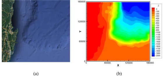
해석 영역은 경도는 129° ~ 131°, 위도 35.1° ~ 36.73°의 지역으로 수심은 약
2,200m(2.2km)이다. 수치 시뮬레이션의 계산 영역은 x, y 및 z 방향으로 각각
180km, 180km 및 2.2km이다. Fig. 9은 해석 영역의 지형의 위성사진과 전처리를
통하여 얻은 수치해석에 사용된 지형을 보이고 있다.
(a) (b)
Fig. 9 Comparison between (a) satellite view and (b) topography data in top view
2. 격자계
가 . 중규모 영역
본 계산을 수행하기 위해 중규모 영역에 대한 격자 수렴도 테스트를 수행하 였다. 수평방향 격자 크기와 개수를 다르게 설정하였고(Table 3), 모든 case에서 수직 방향 격자의 크기와 개수는 동일하게 설정하여(Table 4) 수행하였다(부록 A.
1 참조). 그 결과 중규모 영역에서의 격자를 case 7(80 × 80 × 68, 435,200 개)로 사용하였다(Fig. 10).
Number and sizes(dx) of horizontal(x, y direction) grids
case 1 20/ 9,000m
case 2 30/ 6,000m
case 3 40/ 4,500m
case 4 50/ 3,600m
case 5 60/ 3,000m
case 6 70/ 2,571m
case 7 80/ 2,250m
case 8 90/ 2,000m
case 9 100/ 1,800m
Table 3 Cases for grid dependency test
Number of vertical grids Grid number and water depth Grid sizes(dz)
68
1 ~ 6 (2m ~ -10m) 2m
7 ~ 49 (-10m ~ - 250m) 5m 50 ~ 54 (- 250m ~ - 300m) 10m 55 ~ 56 (- 300m ~ - 400m) 50m 57 ~ 62 (- 400m ~ - 1,000m) 100m 63 ~ 68 (- 1,000m ~ - 2,200m) 200m Table 4 Number of grids and sizes(dz) in z direction for grid dependency tests
(a) (b) Fig. 10 Selected grid system for meso-scale region
(No. of grid in x, y, z direction: 80 × 80 × 68) (a) top ward, (b) perspective views
나. 근방역
근방역 계산 영역은 중규모 영역의 한 개의 격자에 해당하며(Fig 11.), 격자 의 수는 100 × 100 × 45로 전체 450,000개이다(2,250m × 2,250m × 230m). Fig.
12는 중규모 영역에서의 근방역의 위치를 표시한 것과 근방역의 격자에 대한 그 림이다.
Fig. 11 Computed domain of small-scale region in meso-scale region
(a) (b)
Fig. 12 Location of small-scale region in (a) meso-scale region and (b) small-scale region grid
3. 경계 조건
MEC Ocean model은 개방형 경계에 조위나 조류의 속도를 부여하여, 해수
유동을 재현하며, MEC-CO2 model도 동일하다. 본 연구에서는 해석 영역 내 유동 재현을 위해 개방역에 NAO-99jb의 조위 data(Matsumoto et al., 2000) 중 4가지 주 요 조위 성분(Table 5)을 부여하여, 해수 유동을 재현하였고, Hino(1987)의 무반사 조건을 부여하였다.
Tidal Type O1 K1 M2 S2
Period 92,952sec
(25.82h)
86,148sec (23.93h)
44,712sec (12.42h)
43,200sec (12h) Table 5 Tidal components for simulation
또한, 해저면과 해수면에서의 유속에 대해서 No-slip 조건을 적용하였고(식 (29), (30)), 온도, 염분, DCO2은 모든 경계에서 Neumann 조건을 적용하였다(식 (31), 식 (32)).
, (29)
,
(30)
,
,
(31)
, (32)
,
(33)
,
,
(34)
, 은 해저에서의 수평방향 전단응력이며, 는 해저마찰계수이며, 는 수심이 다. 는 온도, 염분, DCO2의 수직 확산 계수(Vertical Diffusivity Coefficient)이다.
, 은 해수면에서의 수평 방향의 전단응력이다. 는 해면마찰계수이다. , 는 해저면에서의 속도이며, , 는 해수면에서의 속도이다.
4. 계산 조건
가 . 온도 , 염분 , 해수 중 용해된 CO
2(DCO
2) 초기조건
Hydrostatic model 영역에 사용된 Scalar 물리량은 우리나라의 얻을 수 있는
자료가 부족하여, 온도, 염분, DCO2의 초기조건은 수심에 따라 Fig. 13와 같이
(Kano et al., 2010) 부여 하였으며 수심 500m 이하의 물리량의 값은 500m와 동
일하게 설정하였다.
Fig. 13 Initial condition (temparature [T], salinity [S], dissolved CO2 [DCO2, C], and density [R])
나 . CO
2누출량 , 누출 비율 및 누출 지점
근방역에서 균열이 발생하여 CO2의 누출이 된다고 상정하였으며, 이때 누출 량은 RITE(The Research Institute for Innovative Techonology for the Earth) 2004에 서 가정한 양을 사용하였다. 누출 지점에서 해수에 용해된 CO2와 CO2 기포의 초 기 누출 비율을 달리하여 해석을 수행하였다(Table 6).
Leakage Amount Initial CO2 bubble ratio case 1
3,800ton/year
10%
case 2 50%
case 3 90%
case 4
94,600ton/year
10%
case 5 50%
case 6 90%
Table 6 Cases of leakage & initial CO2 bubble ratio
근방역 내의 누출 영역은 Fig. 14과 같이 가정하였다. 누출 면적 및 매 초당 CO2 누출량은 각각 50,625m2, 5.9254× ⋅과 2.3802×
⋅이다. 누출되는 기포의 직경은 2cm(0.02m, 반지름 1cm)를 설정하였다.
Fig. 14 Leakage area in small-scale region
다 . 해석 parameter
Table 7은 중규모 영역의 계산과 근방역의 해석에 사용된 계수의 값을 나타 낸 표이다.
수평 와점성 계수(Horizontal Eddy Viscosity)는 Fujino & Tabeta(1991)의 값인 20를 사용하였으며, 수직 와점성 계수(Vertical Eddy Viscosity)는 0.0001
로 사용하였다. 마찰 계수는 0.0025를 사용하였으며, Coriolis 효과는 고려하지 않 았다.
Parameter Value Parameter Value
Time step 1sec Cloud 6.63
Air Density 1.226 Precipitation 0.2743
Water Density 1025 Vapor pressure 26.86 Horizontal Eddy
Viscosity 20 Wind 2.12
Vertical Eddy
Viscosity 1E-4 Air Temperature 26.2℃
Horizontal Eddy
Diffusivity 10 Courant Number 0.5
Vertical Eddy
Diffusivity 1E-5 Diffusive
Number 0.5
Frictional
Coefficient 0.0025
Coriolis
Coefficient 0.0
Table 7 Simulation parameters
제2절 요약
본 장에서 수행한 연구 내용은 다음과 같다.
1) 2017년 CO2 해양지중저장 시험이 수행되었던 포항인근 육지 및 해역 (경
도 129° ~ 131°, 위도 35.1° ~ 36.73°, 180km × 180km, 최대수심 2,200m)을 해석영역으로 선정하였다.
2) 해석 영역의 격자생성에 필요한 육지와 해저지형 정보는 각각 US Geological Survey(USGS)의 GTOPO 30 데이터와 일본해양자료센터(Japan Oceanographic Data Center, JODC)의 데이터를 수집하여 사용하였다.
3) 해석 영역 내 해수유동 재현을 위한 경계조건 부여 및 재현결과 비교를 위해 필요한 조위성분은 NAO-99jb(Matsumoto et al., 2000)와 국립해양조사 원(Korea Hydrographic Oceanographic Agency, KHOA)의 데이터를 이용하였 다.
4) 수집한 조위 성분중 해수유동에 큰 영향을 주는 4개의 분조(O1, K1, M2
& S2)를 선정하였고, 이 4개 분조의 조위성분을 조합하여 개방역의 조위
경계조건으로 사용하였다.
5) 기포 CO2의 용해율 및 국부유동에 영향을 미치는 온도/해수밀도/DCO2의 초기조건 설정을 위하여 관련 데이터를 조사하�