비영리 - S-Space - 서울대학교

(1)

저작자표시-비영리-변경금지 2.0 대한민국 이용자는 아래의 조건을 따르는 경우에 한하여 자유롭게

l 이 저작물을 복제, 배포, 전송, 전시, 공연 및 방송할 수 있습니다. 다음과 같은 조건을 따라야 합니다:

l 귀하는, 이 저작물의 재이용이나 배포의 경우, 이 저작물에 적용된 이용허락조건 을 명확하게 나타내어야 합니다.

저작권법에 따른 이용자의 권리는 위의 내용에 의하여 영향을 받지 않습니다. 이것은 이용허락규약(Legal Code)을 이해하기 쉽게 요약한 것입니다.

Disclaimer

저작자표시. 귀하는 원저작자를 표시하여야 합니다.

비영리. 귀하는 이 저작물을 영리 목적으로 이용할 수 없습니다.

변경금지. 귀하는 이 저작물을 개작, 변형 또는 가공할 수 없습니다.

(2)

도시계획학 석사학위논문

Structural Causes for

the Peak Car Travel in Korea

국내 도로 통행 정점의 구조적 원인 연구

2014 년 7 월

서울대학교 환경대학원 환경계획학과 교통관리전공

송 민 수

(3)

(4)

지도교수 장 수 은

이 논문을 도시계획학 석사학위논문으로 제출함 2014 년 4 월

서울대학교 환경대학원 환경계획학과 교통관리전공

송 민 수

송민수의 도시계획학 석사학위논문을 인준함 2014 년 7 월

위 원 장 (인)

부위원장 (인)

위 원 (인)

(5)

ABSTRACT

Advised by

Prof. Chang, Justin Sueun

Submitted by Song, Minsu

April, 2014

Department of Environmental Planning Graduate School of Environmental Studies

Seoul National University

(6)

Abstract

According to researches conducted by leading European countries, the growth of vehicle traffic in advanced countries whose economic developments have reached a plateau tends to slow down and even decline in some countries(particularly several metropolitan area) as they entered upon 2000s. That is, it takes on an a similar aspect to the growth curve model, which predicts the demand changed by the elapse of time. According to the growth curve model, a growth curve goes through the introductory period where it is slow and the growth period where it is exceedingly steep.

Then, the curve becomes saturated at the maturation period and soon starts to decline slightly at the decreasing period. The predominant view nowadays is that the vehicle traffic in advanced economies is undergoing the maturation period, called 'Peak Car Travel'.

These countries show common changes in varied aspects and they are assumed to be the cause of the peak car. Among those changes are a low growth(a stabilization of economy), a slowdown of population growth, the worldwide economic problems(the rise of gasoline price, etc.) and they are generally regarded as the cause of the peak car in most researches. The change of transportation policy or environment which includes the increase of people who use public transportation, and the tendency of promoting walking and riding bicycles is also commonly suggested. Besides, transition of personal lifestyle preferences such as the tendency of owning cars, the development of Internet-based social network, the generalization of e-commerce and the actualization of remote working are brought up as well.

However, researches relevant to these common changes neither investigate in which direction nor how much they affect the peak car trend

(7)

respectively. Namely, those researches discuss the correlation between the statistically analyzed changes and peak car trend qualitatively, but do not present the cause-and-effect quantitatively. Thus, the current study aims to answer the following questions:

1) Does the vehicle traffic of Korea show the peak car trend in a similar way to advanced countries?

2) If so, what is the quantitative and structural causes of it? How much do they work on it?

One of the generally used units of analysis vehicle traffic is the Vehicle Kilometer Travelled. In this study, considering the object and the scope of the study, yearly total VKT per capita for private car by region estimated from daily average VKT data by Korea Transportation Safety Authority was used as an index of vehicle use volume. Also, after reviewing and categorizing preceding researches, this study formed a set of explanatory variables which has suitability considering the current state of Korea. Based on this, this study assessed prime predictors using the Structural Equation Model. The Structural Equation Model is a model composed of the confirmatory factor analysis based on the theory developed in the field of praxeology and multiple regression analysis developed in the field of econometrics. Therefore, the Structural Equation Model is appropriate for the case where combined influence of large number of factors causes the social multiple symptoms.

The major findings of this study are as follows. First, Korea has also shown the peak car trend similar to those of European countries, and the

(8)

quantitative values are alike as well. Daily average distance traveled per vehicle within investigated sample shows a definite decline, and the estimated VKT based on this tends to level off. Secondly, among four latent variables that affects the peak car, economic factor has largest carrying capacity, and then transport factor, land use factor and lifestyle factor by order. GRDP and gasoline price are identified as a economic factor significantly associated with the peak car. Public transportation is significant transport factor predicting the peak car. Social ageing and female rate of economically active population were shown to be the factor that predicts the peak car trend meaningfully. This indicates that higher income, low gasoline price, less public transport-oriented, not being under social ageing, lower rate of female who are economically active were associated with bigger vehicle traffic volume. In Korea's case, it can be said that we have met or are meeting the conditions mentioned above. As a result, the slowdown in growth(or an absolute decline) of vehicle traffic is predicted to last in the future.

The peak car trend implies the decrease of car dependence, so the general and dominant view toward the future growth potential of the car use which have even been taken for granted for decades cannot subsist anymore.

Since a great deal of transportation plans and policies is based on the prediction of future growth, the possibility of stagnation or even a meaningful decrease carries a heavy significance. The peak car trend suggests a potential change of the analysis and the prediction of the demand of road traffic, and thus can function as a criteria for decision making for when and how much to invest in facilities and services. Therefore, if sociocultural features that affects the peak car trend, including factors that were found meaningful in this study, are applied to the analysis for the

(9)

demand of road traffic, policy makers may be able to cope with the change of the demand in a more anticipative way. Above this, as a context of environmentally sustainable transportation, primary issue for now and the upcoming era, the peak car trend can perform a role as a grounds for the policy of car diminution.

There are currently uncertainties in judgement on whether the observed trends are transitory or a permanent change, and on what kind of aspect it heads toward. Above this, the factors that was originally meant to be treated weighty show low significance probability, which is considered to partially results from limitation of the panel data. If subsequent studies is being conducted by constructing the questionnaire that was structured to meet the purposes of the study, it will be able to construct more accurate model, complementing the limitation of aggregate secondary data presented in this study. It can also be possible to construct different models by regional groups or urban community types. Lastly, constructing available model for developing countries on growth in demand for road traffic is expected to contribute to the establishment of more advanced transport policy by predicting certain time or relevant demand for the peak car.

Key Words : Peak car, Total vehicle kilometer traveled, Structural Equation Modeling, Factor loading, Transportation policies Student Number : 2011-23926

(10)

LIST OF TABLES

<Table 1> Summarize of studies on supposed factors for peak car ···· 11

<Table 2> Fit indices and their acceptable thresholds ··· 25

<Table 3> Detailed notion and definition of relevant factors ··· 35

<Table 4> The descriptive statistics of economic factors ··· 43

<Table 5> Missing Rate and Normality of the Study Variables ··· 45

<Table 6> Pearson Correlation Coefficients ··· 46

<Table 7> Predictors of the peak car ··· 47

<Table 8> Predictors of the peak car ··· 49

<Table 9> Acceptance range of Goodness-of-fit and fit index of the model ··· 50

<Table A> Daily average distance traveled per vehicle within investigated sample (km) ··· 57

<Table B> Yearly total vehicle kilometer travelled for all vehicle types(million km) ··· 58

<Table C> Yearly total vehicle kilometer travelled per capita for private car(km) ··· 59

(13)

LIST OF FIGURES

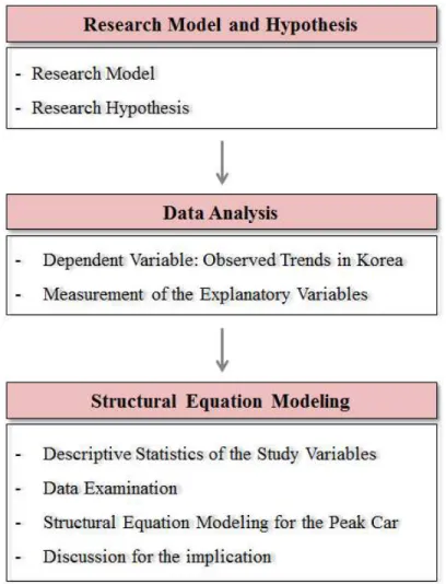
<Figure 1> Research flow of this study ··· 5

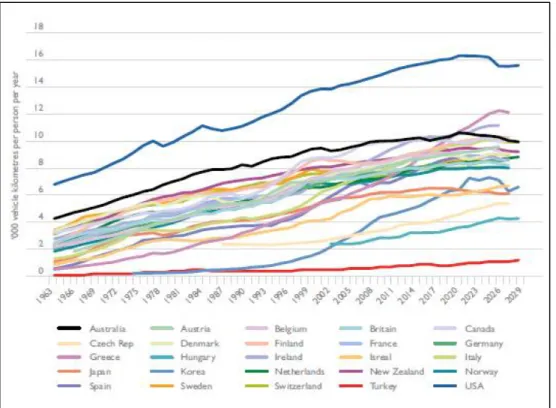
<Figure 2> Patterns of traffic per person in 25 countries ··· 7

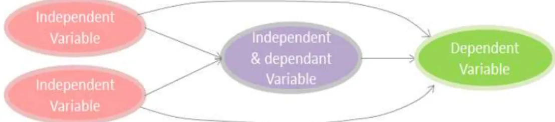
<Figure 3> Relationship among Variables in SEM ··· 13

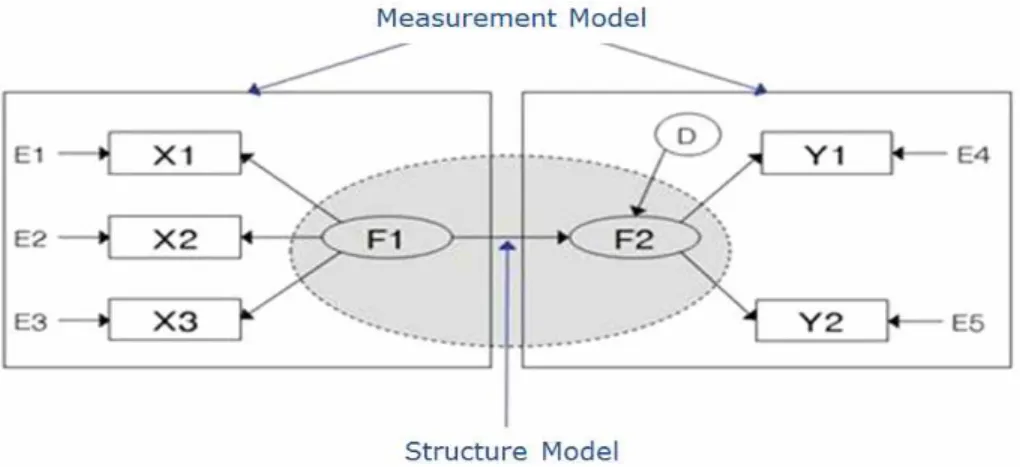
<Figure 4> Measurement model and Structure model ··· 15

<Figure 5> General form of the path diagram of SEM ··· 16

<Figure 6> Process for VKT data collection(2012) ··· 29

<Figure 7> Daily average distance traveled per vehicle within investigated sample for all vehicle types and private car ··· 30

<Figure 8> Path diagram for the hypothetical model ··· 42

<Figure A> Daily average distance traveled per vehicle within investigated sample(km) ··· 60

<Figure B> Yearly total vehicle kilometer travelled for all vehicle types(million km) ··· 61

<Figure C> Yearly total vehicle kilometer travelled per capita for private car(km) ··· 62

(14)

I. Introduction

1. Background and Purpose

In most developed countries with advanced economies, growth trend of figures like total vehicle use volume, or car use per person, has leveled off since the early 2000s. In some countries it has even declined. After expanding rapidly in the 1960s and 70s, growth in road traffic slowed and seemed to approach the saturation point (Litman, 2009). This trend stresses the need to take account of such other factors as rising fuel prices and the distribution of wealth, as well as the scope of future transport demand trends in the emerging economies.

This study looks into the contribution of various factors to

‘peak car’ in Korea. The term ‘peak car’ was coined to describe recent trend reversal in car travel growth observed in some industrialized countries. That is, ‘peak car’ means car travel trend characterized by growth for a long time but started to show signs of stagnation or even decrease in the last decade.

Then why we have to cognize, or put emphasis on ‘peak car travel’ trend? The statistical facts of a reduction in growth, low growth or stability at national level, and reductions in specific

(15)

locations especially some larger urban areas seem broadly agreed by most analyses. ‘Peak car’ trend is one of those low growth trends.

Phil Goodwin(2012) delineated the significance of ‘peak car travel’ in his research paper as follows:

“Since a very large part of the policy and planning of transport has been based on forecasts of future growth, the possibilities that car use may grow significantly less, stabilize, or reverse, are of profound importance. As a caveat, it should be said that a full analysis of this question really should be located in much wider methodological and empirical issues of travel demand analysis. Such a wider discussion would take on board the multi-disciplinary literatures on demand elasticity, induced and suppressed traffic, and the effects on travel choice, in the short and long run, of infrastructure provision and policy interventions. Of particular importance is the emerging empirical evidence on the impacts of policies aimed at reducing car use such as pricing, pedestrianisation, public transport improvements, cycling, and land-use planning.”

The economic recession and relatively high fuel prices may explain part of the decline in the growth of travel, but not all of it.

What other factors than GDP and fuel prices are making the change in car use growth? Do the trends being observed reflect the approach

(16)

of the saturation point via a decoupling of the growth rates for traffic and income (Millard-Ball and Schipper, 2010)? Is this decoupling manifesting itself first in the most densely populated regions and/or over a certain standard of living? Or does the levelling-off of traffic result rather from a cancelling out of opposite trends(continued growth in rural and suburban areas and decline amongst residents of the most densely populated areas) (Goodwin, 2010)?

Some people posit the assumption of a reduction in travel in the developed countries in the short and medium terms, attributable to a variety of socio-economic factors (Litman, 2011). One could well ask whether this is a socio-demographic phenomenon (population ageing, re-densification of large city areas, fewer but more-intensive workdays, etc.) or an economic one linked to rising and volatile fuel prices and the recession (Gardes et al., 1996).

Understanding the determinants of aggregate volumes of vehicle use, and particularly of changes in the weight or the nature of such determinants, is of interest to policy-makers and to industry.

Designing mobility policies, including but not limited to planning infrastructure development, requires forward-looking analysis of the demand for mobility. It can help to making supply plans about road traffic more precise and accurate. If it turns out that the drivers of demand are changing, projection methods need to be revised.

This study is not expected to contribute limitedly to transport in a narrow sense. If car use is likely to grow more slowly than in the past, this may affect decisions on land-use, on environmental and

(17)

climate change policy. Therefore, defining key factors and relationships among the factors for the growth saturation can contribute to national weighty policies and enables making provision for the upcoming era.

2. Scope and Method

In this study, vehicle kilometer traveled is measured as the indicator for the vehicle travel volumes. Many different studies have used different methodologies and definitions, but it has been observed that car use, or total car traffic, or road total traffic are shown by vehicle kilometer traveled(or that per capita) or passenger kilometer traveled(or that per capita). In a few countries, there have been similar studies of the distance travelled by all modes added together, which have shown a similar trend in terms of national travel.

Considering availability of data, this study analyses vehicle kilometer traveled and car kilometer. Comparison among total vehicle kilometer traveled, that per household, and that per capita will be shown in Chapter Ⅲ-1.

The study is conducted by the form of panel data. For the time-series, the data from 2000 to 2012(13 years) is used, and the data based on province level(16 provinces) is used for the cross-section analysis. Therefore, 208 of observation points are collected and comprise this study.

(18)

3. Structure of Thesis

A simple flow of this study is shown in Figure 1.

Figure 1. Research flow of this study

(19)

Ⅱ . Advanced Research and Literature Review

The principal objective of this study is to provide policy implications regarding methods by which government policy makers can formulate policies related to new trends of peak car. This work is constructed on the basis of quantitative and qualitative exploration of various factors. The qualitative methods are used in the theoretical part and the quantitative analysis is used for empirical analysis part. The research starts by reviewing the related literature on peak car travel, and structural equation modeling(SEM). The bases of the analysis depend on the dataset, which is explained in Chapter Ⅳ of this thesis.

1. Analysing Worldwide Trends

1) Aggregate Observed Trends at National Level

According to Bureau of Infrastructure, Transport and Regional Economics (BITRE) Australia, in Australia as other countries around the world, traffic growth has been a feature of the post World War Two experience. The automobile and commercial vehicles have multiplied, as living has increasingly been intertwined with mobility.

BITRE(2012) examined the trends in the growth of road

(20)

traffic(vehicle kilometers travelled) in 25 countries around the world, from 1963 to 2010. Some countries experienced an early period of faster growth in traffic. On the other hand, after rapid growth in the sixties and seventies, the levelling-off, or deceleration in traffic growth is apparent in several countries. In addition, Australia, the United Kingdom and the USA seemed to decline since around 2005. The main results of this study are models of VKT per capita as a function of real petrol prices, fluctuations in the economy and of a saturating effect of time.

Figure 2. Patterns of traffic per person in 25 countries Source: BITRE(2012)

(21)

An early piece of research to speculate that a levelling off of growth was occurring on an international scale was by Schipper et al.(1993), and he continued this work until in 2010. It included some influential and often cited graphs on 8 industrialised countries. In 2011, the International Transport Forum showed similar figures.

Despite those international signs show a substantial variation, there’s no doubt but it seems to be a widespread phenomenon. Accordingly, many studies have suggested various factors for this phenomenon.

2) Diagnosis of Factors

The impact of various socio-demographic characteristics on travel demand can be described as a factors for ‘peak car’. It is generalizations and simplifications of empirical observations which are not valid for all specific cases, but intended to capture average or regularities.

Kuhnimhoff et al.(2012) provide a systematic comparison of six countries; France, Germany, UK, Japan, Norway, USA. Travel survey data on 1995 and 2005 are used for the study. In itself, population ageing has a negative impact on car travel in all studied countries. However, the negative effect of ageing is counteracted by the increase in car ownership at higher age in all studied countries except for the USA. Car ownership among young adults has declined in Norway, the UK, Germany, and the USA. In the middle age

(22)

groups, there were declines in Germany and the USA and increases elsewhere. Reduced car ownership among young adults is key to explaining the aggregate pattern in Germany, the UK, and Norway.

The effect of mode choice differs between countries. In Germany and the UK, modal shifts away from the car contribute strongly to reduced car use. In japan the effect is small, and in France and Norway there was a shift in the reverse direction.

According to Le Vine and Jones(2012), the number of car trips, their length, and occupancy rates were roughy constant from 1995 to 2007. With comparison of British travel survey data of 1995, 2000, and 2005, travel declined most for the young men. For women aged 20 to 29 travel was stable, and it increased most strongly for the oldest. There is also evidence that persons born outside the UK travel less than those born in the UK. The decline of car driving over time is visible in all income brackets except the lowest, and is stronger as income is higher. Nevertheless, higher incomes remain associated with more driving. The largest decline in car travel is for shopping and visiting friends and relatives.

Van der Waard et al.(2012) shows that total car kilometers by drivers leveled off since 2005, and car kilometer by passengers declined. Car ownership kept rising and so did license-holding excepts for 25~29 year olds. Mobility among young adults fell notably for 18~29 year olds, and more moderately for 30~39 year olds. This is both because of group size and changes in group behavior. Men aged 18~29 travelled 16% less in 2009 than in 1995 while women

(23)

travelled 6% more. These changes appear to be linked to strong reurbanisation and to a rising share of students and declining share of workers in this age bracket. Their cheap public transport might have a substantial affect on students’ travel choices. There is no evidence of a shift in preferences for car towards smartphones or tablet computers.

For the USA, Davis et al.(2012) emphasize the role of young adult’s travel choices in explaining the observation that per capita car travel started declining in 2004. Household travel survey data show that per capita car travel in the age group 16~34 fell by 23%

between 2001 and 2009. The share of 14~34 year olds without a license increased from 21% to 26% over same period. Increased use of other modes suggests a degree of substitution, and this substitution is facilitated by increased urban living. Within urban areas real estate development and land use patterns are changing, with less urban fringe and car-oriented development. Furthermore, Barriers to driving, including high gas prices and tougher licensing laws matter too.

Madre et al.(2012) emphasize contrasting developments between large urban areas and less dense regions. in France In large urban areas, fewer car trips were made per person in 2004 than in 1998. In lower density regions, there are more cars and they are used for longer trips. Car ownership declined, and there was a slight decline in license-holding among young adults. These changes took place irrespective of income levels. Fuel prices increases around 2000 play a role in explaining the declining growth rate.

(24)

Country Measurement

for peak car Methodology Observed factors related

Kuhnimhoff et al.(2012)

France, Germany, UK, Japan, Norway, USA

car kilometers per

tripmaker(age 20 and over)

comparison of the descriptive analysis result

age distribution, car ownership, vehicle mode share

Le Vine and Jones(2012)

UK

car kilometers per capita

descriptive analysis with travel survey data

age distribution, gender, income, travel purpose, company car use(case of London) Table 2. Summarize of studies on supposed factors for the peak car

Hyodo(2012) shows that car kilometers in Japan fell as of 1999, as a result of shorter trips and despite an increase in the number of trips and passengers. Low growth, translating particularly into rising numbers of low income households, and high gas prices drive part of this result. Other changes, including later age of marriage, smaller households, and population ageing and a decline of the total population(since 2009) work in the same direction. Fewer younger drivers and decline of younger female drivers is pronounced.

To summarize, various factors for measurement from former studies are as follows(Table 1). They observe aggregative tendency and suppose it to be the causes for peak car, but do not define how much on which direction it occurs.

(25)

Van der Waard et al.(2012)

Netherlands

person kilometers, car kilometers per person

descriptive analysis

car ownership, driver license holding, travel purpose,

re-urbanisation, income, labour participation by women, changing in travel times, changing mobility of young adults, internet based society, increased international mobility

Davis et

al.(2012) USA

car kilometers per person

age distribution, driver license holding, mode share, increased urban living

Madre et

al.(2012) France car trips per person

urbanisation, car ownership, Fuel price, income, population density

Hyodo

(2012) Japan

vehicle kilometer per person, passenger kilometers

car ownership, license holding, population size, ageing rate, number of households, marriage age, gas price, GDP growth rate, income, travel time

(26)

2. Review of Structural Equation Model

Structural equation model(SEM) is the methodology that multivariate regression model, or path analysis, and confirmatory factor analysis, based on measurement theory from sociology and psychology, are combined (Bae, 2011). It is appropriate for the research that combined influence of large number of factors causes certain social multiple symptoms (Fox, 2002).

Unlike the more traditional multivariate linear model, the response variable in one regression equation in a SEM may appear as a predictor in another equation. Indeed, variables in SEM may influence one-another reciprocally, either directly or through other variables as intermediaries. These structural equations are meant to represent causal relationships among the variables in the model. In this case, the factors have a large number of sub-variables.

Figure 3. Relationship among variables in SEM

(27)

A model of factor analysis and path analysis into one comprehensive statistical methodology is referred to as structural modeling (Kaplan, 2000). SEM is a comprehensive statistical approach, and it evaluates the hypothesis in relation to the latent variables and the observed variables (Hoyle, 1995). SEM enables researchers to answer a set of interrelated questions within a single, systematic, and comprehensive analysis by simultaneously modeling the relationships among multiple independent and dependent constructs (Gerbing and Anderson, 1988). This is a viable multivariate tool, and has been utilized by communications researchers for the past quarter-century; however, it can also be employed in different fields of study, including economics, biology, marketing science, and medical science (Tenko and Marcoulides, 2000). SEM generally incorporates latent variables which cannot be measured directly. According to the seminal work conducted by Joreskog and Van Thillo in 1972 (Yevette and Lindsay, 1999), SEM began as a tool for inspecting the relationship between unobserved latent variables and observed variables.

The SEM technique was derived from the following three separate lines of mathematical and statistical analysis: (1) path analysis, (2) factor analysis, and (3) simultaneous equation modeling.

Path analysis is commonly attributed to Wright(1934), who demonstrated the manner in which correlations among variables might be associated with the parameters of the represented model. While Wright was refining his path analysis method, Thurstone(1947) was

(28)

advancing his approach to factor analysis. Similarly, individuals conducting research in the field of econometrics began to refine the simultaneous equation modeling technique.

The SEM begins with model specification, as per the researchers’ expectations, in order to estimate what type of relationship actually exist between latent variables and observed variables. Here, the latent variables represent the theoretical or hypothetical constructs of the researchers¹⁾ (Christoper, 1999). These two variables are connected by arrows, which may be one-way or two-way, based on the researcher’s hypothesis or the theoretical plan.

A one-way arrow represents the path and two-way arrows refer to the correlation between two variables (Tenko and Marcoulides, 2000).

Figure 4. Measurement model and Structure model

1) The latent variables are presented in circles or ellipses whereas observed variables are number or fact presented in rectangles.

(29)

The SEM model contains two interrelated models: the measurement model and the structural model. Both models are defined explicitly by the researchers. The measurement model defines the constructs(latent variables) in the model we use herein, and assigns observed variables to each. The structure then defines the causal relationship among the latent variables. The measurement model employs factor analysis to evaluate the degree to which the observed variables load on their latent constructs.

1) Path Diagram of SEM

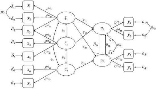
Figure 5. General form of the path diagram of SEM

Figure 5 is a general form of the path diagram of SEM. Rectangle form is for the observable variables, while oval form is for

(30)

non-observable ones. In addition, single arrow means direct causal relationship between two components, and arrow towards both sides means interrelation.

2) Mathematical Formulation of SEM

The structural equation model can be expressed generally in terms of the LISREL model, which was introduced by Joreskog in 1972 and refined by Fox(2002), in drawing the path diagram:

 represents observable exogenous variables. If there were latent exogenous variables in the model, these would be represented by ’s, and ’s would be used to represent their observable indicators.

’s are employed to represent the indicators of the latent endogenous variables, which are symbolized by ’s. If there were directly observed endogenous variables in the model, then these two would be represented by ’s. ’s and ’s are used, respectively, for structural coefficients relating endogenous variables with exogenous variables and to one another, and ’s are utilized for structural disturbances. The parameter, _, represents the covariance between the disturbances _ and _.

In the measurement sub model, ’s represent the regression coefficients relating the observable indicators to the latent variables.

(31)

The superscript  in ^ shows that the factor loadings in this model pertain to indicators of latent endogenous variables.

The ’s represent the measurement error in the endogenous indicators; if there were exogenous indicator in the model, then the measurement errors associated with them would be represented by ’s.

The SEM is expressed as follows:

_ _ _ _

_ __ _ ………(Equation 1)

_ __ _

Identifying many of the parameters in Equation 1 requires that some of the parameters are typically set to 0 or 1, or defined as equal.

Unknown parameters can be estimated by the dataset, in which a positive sign signifies that the observed variable(or latent variable) positively affects the latent variable(or the observed variable). As the former increases, in other words, the latter also increases. This relationship can be observed among the whole variables, including the observed variables and latent variables. Path analysis distinguishes three types of effects: direct, indirect, and total effects. The decomposition of effects always occurs with regard to a specific model. If the system of equation is altered via the inclusion or exclusion of variables, the estimates of total, direct, and indirect effects may change.

(32)

3) Evaluating Goodness-of-fit of SEM

However the issue of how the model that best represents the data reflects underlying theory, known as model fit, is by no means agreed. It is essential that researchers using the technique are comfortable with the area since assessing whether a specified model

‘fits’ the data is one of the most important steps in structural equation modelling (Yuan, 2005).

The following description about classification and recommendation of fit indices are extracted and summarized from the Guideline for determining model fit (D. Hooper et al., 2008).

(1) Absolute fit indices

Absolute fit indices determine how well an a priori model fits the sample data (McDonald and Ho, 2002) and demonstrates which proposed model has the most superior fit. These measures provide the most fundamental indication of how well the proposed theory fits the data.

a) Model chi-square (^)

The Chi-Square value is the traditional measure for evaluating overall model fit and, ‘assesses the magnitude of discrepancy between the sample and fitted covariances matrices’ (Hu and Bentler, 1999: 2).

(33)

A good model fit would provide an insignificant result at a 0.05 threshold (Barrett, 2007), thus the Chi-Square statistic is often referred to as either a ‘badness of fit’ (Kline, 2005) or a ‘lack of fit’ (Mulaik et al, 1989) measure. While the Chi-Squared test retains its popularity as a fit statistic, there exist some limitations in its use. Where small samples are used, the Chi-Square statistic lacks power and because of this may not discriminate between good fitting models and poor fitting models (Kenny and McCoach, 2003).

b) Root mean square error of approximation (RMSEA)

The RMSEA is the second fit statistic reported in the LISREL program and was first developed by Steiger and Lind (1980, cited in Steiger, 1990). The RMSEA tells us how well the model, with unknown but optimally chosen parameter estimates would fit the populations covariance matrix (Byrne, 1998). Recommendations for RMSEA cut-off points have been reduced considerably in the last fifteen years. Up until the early nineties, an RMSEA in the range of 0.05 to 0.10 was considered an indication of fair fit and values above 0.10 indicated poor fit (MacCallum et al., 1996). However, more recently, a cut-off value close to .06 (Hu and Bentler, 1999) or a stringent upper limit of 0.07 (Steiger, 2007) seems to be the general consensus amongst authorities in this area.

(34)

c) Goodness-of-fit statistic (GFI) and the adjusted goodness-of-fit statistic (AGFI)

The Goodness-of-Fit statistic (GFI) was created by Jöreskog and Sorbom as an alternative to the Chi-Square test and calculates the proportion of variance that is accounted for by the estimated population covariance (Tabachnick and Fidell, 2007). By looking at the variances and covariances accounted for by the model it shows how closely the model comes to replicating the observed covariance matrix (Diamantopoulos and Siguaw, 2000). This statistic ranges from 0 to 1 with larger samples increasing its value. It has also been found that the GFI increases as the number of parameters increases (MacCallum and Hong, 1997) and also has an upward bias with large samples (Bollen, 1990; Miles and Shevlin, 1998). Traditionally an omnibus cut-off point of 0.90 has been recommended for the GFI however, simulation studies have shown that when factor loadings and sample sizes are low a higher cut-off of 0.95 is more appropriate (Miles and Shevlin, 1998).

Related to the GFI is the AGFI which adjusts the GFI based upon degrees of freedom, with more saturated models reducing fit (Tabachnick and Fidell, 2007). AGFI tends to increase with sample size. As with the GFI, values for the AGFI also range between 0 and 1 and it is generally accepted that values of 0.90 or greater indicate well fitting models.

(35)

d) Root mean square residual (RMR) and standardised root mean square residual (SRMR)

The RMR and the SRMR are the square root of the difference between the residuals of the sample covariance matrix and the hypothesised covariance model. The range of the RMR is calculated based upon the scales of each indicator, therefore, if a questionnaire contains items with varying levels (some items may range from 1~5 while others range from 1~7) the RMR becomes difficult to interpret (Kline, 2005). The standardised RMR (SRMR) resolves this problem and is therefore much more meaningful to interpret. Values for the SRMR range from zero to 1.0 with well fitting models obtaining values less than .05 (Byrne, 1998;

Diamantopoulos and Siguaw, 2000).

(2) Incremental fit indices

Incremental fit indices, also known as comparative or relative fit indices, are a group of indices that do not use the chi-square in its raw form but compare the chi-square value to a baseline model. For these models the null hypothesis is that all variables are uncorrelated (McDonald and Ho, 2002).

(36)

a) Normed-fit index (NFI)

The first of these indices to appear in LISREL output is the Normed Fit Index (NFI: Bentler and Bonnet, 1980). This statistic assesses the model by comparing the ^ value of the model to the

^ of the null model. Values for this statistic range between 0 and 1 with Bentler and Bonnet (1980) recommending values greater than 0.90 indicating a good fit. A major drawback to this index is that it is sensitive to sample size, underestimating fit for samples less than 200 (Mulaik et al., 1989; Bentler, 1990).

b) CFI (Comparative fit index)

The Comparative Fit Index (CFI: Bentler, 1990) is a revised form of the NFI which takes into account sample size (Byrne, 1998) that performs well even when sample size is small (Tabachnick and Fidell, 2007). As with the NFI, values for this statistic range between 0.0 and 1.0 with values closer to 1.0 indicating good fit. A cut-off criterion of CFI ≥ 0.90 was initially advanced however, recent studies have shown that a value greater than 0.90 is needed in order to ensure that misspecified models are not accepted (Hu and Bentler, 1999). From this, a value of CFI ≥ 0.95 is presently recognised as indicative of good fit (Hu and Bentler, 1999). Today this is included in all SEM programs and is one of the most popularly reported fit indices due to being one of the measures least effected by sample size (Fan et al, 1999).

(37)

(3) Parsimonious fit indices

Having a nearly saturated, complex model means that the estimation process is dependent on the sample data. This results in a less rigourous theoretical model that paradoxically produces better fit indices (Mulaik et al., 1989; Crowley and Fan, 1997). To overcome this problem, Mulaik et al.(1989) have developed two parsimony of fit indices; the Parsimony Goodness-of-Fit Index (PGFI) and the Parsimonious Normed Fit Index (PNFI). The PGFI is based upon the GFI by adjusting for loss of degrees of freedom. While no threshold levels have been recommended for these indices, Mulaik et al.(1989) note that it is possible to obtain parsimony fit indices within the .50 region while other goodness of fit indices achieve values over .90 (Mulaik et al., 1989).

(38)

Fit Index Acceptable Threshold Levels Description Absolute Fit Indices

Chi-Square(^)

Low ^ relative to degrees of freedom with an insignificant p value (p > 0.05)

Adjusts for sample size

RMSEA 2:1 (Tabachnik and Fidell, 2007) 3:1 (Kline, 2005)

Values less than 0.03 represent excellent fit GFI/AGFI Values greater than 0.95

Scaled between 0 and 1, with higher values indicating better model fit RMR/SRMR

Smaller is the better(RMR) Unstandardised

less than 0.08(SRMR) Standardised version of the RMR

Incremental Fit Indices

NFI values greater than 0.95

Assesses fit relative to a baseline model which assumes no covariances between the observed variables. Has a tendency to overestimate fit in small samples

CFI values greater than 0.95 Normed, 0~1 range Table 3. Fit indices and their acceptable thresholds

(39)

Ⅲ . Data Analysis

1. Dependent Variable: Observed Trends in Korea

1) Basic Information on Data

The main database used for this thesis is the kilometrage of vehicles created and annually updated by the Korea Transportation Safety Authority.

The kilometrage of vehicles is thought of as one of 557 evaluation factors with which IRTAD(International Road and Traffic Accidents Database) rates OECD members by means of international competitiveness and traffic safety level annually(Korea Transportation Safety Authority, 2012). In addition, the kilometrage of vehicles is used for development of plans for road safety, decision of traffic policies, making standards for the imposition of environmental improvement contributions, the calculation of the greenhouse gas emissions, and training materials for the transportation companies.

At 1985 Korea has set to investigate the kilometrage of vehicles for the first time, thereafter being done at unevenly-spaced intervals, since 1999 up to the present time it keeps estimating the annual kilometrage of vehicles that is used for various purposes.

(40)

Traffic Volume (VKT) = Number of Vehicles * Distance Travelled

= VKT per person * number of people

VKT measures the total distance traveled by all vehicles and treats a kilometer travelled by a car. It is the best available general measure of traffic volume. The estimation of VKT has been required for planning purposes, environmental monitoring, accident analysis, highway fund allocation, and estimation of vehicle emissions. In addition, VKT is a widely used international proxy for the pressures of road transport on the environment and human health(BITRE, 2012).

VKT estimates can also contribute information necessary to inform infrastructure investment decisions and road safety policy(BITRE, 2010). Due to its high impact on policy decisions, it is critical to be able to measure, model and forecast traffic growth, as represented by VKT.

For the estimation of VKT, vehicles under obligation to undergo an automobile inspection from January to December each year were collected. The vehicles under obligation are classified by usage(official, business, and private), by vehicle type(car, van, truck, and special automobile), by fuel(gasoline, diesel, and LPG). Besides, as a mean of reliability checking, two data sets extracted from the total set of vehicles examined are rated as around 0.1% in order to make better the sampling process. By the use of SQL(Structured Query Language) the data of VKT were tabulated(Korea Transportation Safety Authority, 2005). Supposing a sample of 3,000

(41)

vehicles yearly average, the sampling error moves around 0.01%, which is effective for both cases(a total set, 2 alternative sets), hinting at that the reliability and the representative problem can be solved within this sampling size(Choi, 2005).

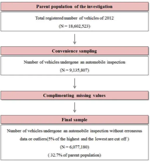
The parent population of inquiry is total vehicle registered in the Ministry of Land, Infrastructure and Transport. Then the vehicles investigated in automobile inspection on each year are defined to be the convenience sample. In the case of 2012, 6.07 million vehicles are used for the convenience sample. This is about 32.7% of total registered vehicles. Samples are classified with vehicle type, fuel type, and usage. Then daily average VKT of samples for each year is calculated, and yearly total VKT is calculated by multiplying the registered number of vehicles²⁾ for relevant year. Process for data collection in case of 2012 is as follows (Figure 6).

2) Registered number of vehicles at June 30 for relevant year is regarded to represent the yearly registered vehicles.

(42)

Figure 6. Process for VKT data collection(2012)

(43)

2) Changing Trends of the Vehicle Kilometer Traveled in Korea

According to daily average distance traveled per vehicle within investigated samples from the Korea Transportation Safety Authority, similar tendency with other 25 countries in advanced economies dealt with in BITRE(2012) got visually and intuitionally captured (Figure 7 and Attached Table A).

It has generally decreased from 1984 to 2012 in every types and usages, and whole group average. The whole group average has dropped off by about 30 percent in the same period, and private car decreased constantly.

Figure 7. Daily average distance traveled per vehicle within investigated sample for all vehicle types and private car

(km)

(44)

However, it cannot be said that the data of daily average distance traveled per vehicle within investigated samples exactly reflect real situation. The reasons are as follows. First, it cannot represent the traffic demand from overall view because continuously increasing number of vehicles registered is not reflected. In addition, as a result from growth of average income of household, it is natural that daily average distance travelled per vehicle has constantly decreased because of increased number of vehicles per household. Consequently, to make an appropriate diagnosis for real state from the aspect of traffic demand, it is more reasonable to analyse this on the basis of total VKT data.

At the initiatory stage, two aspects of VKT are considered on this thesis. One is for all types of vehicle, the other is only for private cars. However, the former is not suitable in terms of the purpose of the research because it consists of all types of vehicles which have significantly different travel characteristics. For this reason, data for the trend of private car only is separately considered. It is directly concerned with the scope and purpose of factors this research focuses on, and also has semantic correlation with explanatory variables. And to conclude, data for the trend of private car make it possible to make a relatively accurate judgement.

It's necessary to examine VKT by regional groups, because it shows different aspect by regions that have different socioeconomic characteristics. Regional VKT data are examined by 3 different types - total, per household, and per capita. But total VKT understandably

(45)

increase because of its calculation process³⁾. To exclude this bias, VKT per household or per capita is rather appropriate instead of total VKT. VKT per household can exclude the impact of increasing number of household, and VKT per capita doesn't include that of population.

As a result of comparison, all possible dataset types seem to have analogous shape one another. Thus, it might well not be unreasonable that this is a nationwide and general trend, which means each figure can be used as a dependent variable of empirical study or quantitative modeling. However, dependent variable must be semantically related to the explanatory variables to meet the purposes of the study. Explanatory variables of this study are intended to be focused on personal propensity and lifestyle change, total VKT per capita for private car is set for the final dependent variable(see Attached Table C and Figure C).

3) Increase of total VKT directly includes increase of registered vehicles, which intuitionally results from increasing number of household and population.

(46)

2. Measurement of the Explanatory Variables

The result of collecting and categorizing all the factors referred to in the previous studies mentioned above. On this basis, items which are strongly correlated in semantic with each other is are integrated or removed to avoid overlapping. Given the characteristics of the data of this study⁴⁾, unavailable data are unavoidably removed as well.

Furthermore, data which is in accordance with study purpose and can reflect our actual situation are added. As a result of the above process, the final composition of variables are set.

1) Latent Variables

Latent variables are composed of economic factor, transport factor, land use factor and lifestyle factor.

2) Observed Variables

GRDP(Gross Regional Domestic Product), gasoline price, car insurance cost compose the economic factor, and public transport, traffic accident, parking area are components of transport factor. Land use factor includes urbanization index and urbanized area, while ageing, licence age, female labor market participation, necessary travel time

4) All items must have data which are constructed annually, and available by region at the relevant years.

(47)

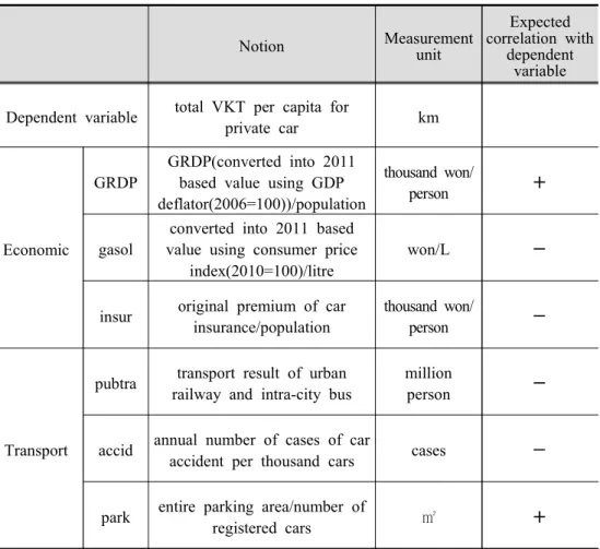
Notion Measurement unit

Expected correlation with

dependent variable Dependent variable total VKT per capita for

private car km

Economic

GRDP

GRDP(converted into 2011 based value using GDP deflator(2006=100))/population

thousand won/

person ＋

gasol

converted into 2011 based value using consumer price

index(2010=100)/litre

won/L －

insur original premium of car insurance/population

thousand won/

person －

Transport

pubtra transport result of urban railway and intra-city bus

million

person －

accid annual number of cases of car

accident per thousand cars cases －

park entire parking area/number of

registered cars ㎡＋

Table 3. Detailed notion and definition of relevant factors

compose the lifestyle factor. At first gender ratio is considered as one of the factors, it is resultingly removed after examining multicollinearity. It is shown that gender ration and female labor market participation have multicollinearity, with variance inflation factor value(VIF) 12.640, 14.449. When VIF is over 10, the existence of multicollinearity has to be considered.

Detailed notion and definition of each factor can be found in Table 3 below.

(48)

Land use

urban

standardized sum of population density, birth rate,

college graduate rate

ㅡ －

urbare build-up area/entire area % －

Lifestyle

&

preferences

ageing portion of the population

aged over 65 % －

licen license acquisition age age －

ecofe

female proportion of economically active

population

% －

necetra

the time required for commute to work or

school(factor for housing-and-jobs proximity)

min. ＋

Note. gasol: gasoline price; insur: car insurance cost; pubtra: public transport; accid:

traffic accident; park: parking area; urban: urbanization index; urbare: urbanization area; licen: license age; ecofe: female rate of economically active population;

necetra: necessary travel time

(49)

3. Data Analysis Procedure

The aim of this study is to identify factors associated with the peak car trend in Korea with the specific focus of exploring the change of lifestyle and preferences in predictors. Data taken from the annual automobile inspection by the Korea Transportation Safety Authority, and from a number of relevant institutions were analyzed according to the procedures presented in this section.

First, descriptive analyses were performed to identify characteristics of explanatory variables. The weighted values are recommended to be reported along with descriptive statistics to estimate the characteristics of the national population from the sample employed in certain study, but this study don’t need them because of the type of panel data.

Second, Examined in this step as well were missingness, normality of data, and multicollinearity to observe whether distributions of study data were adequate for analysis with structural equation modeling (Bae, 2009).

Third, data analysis using structural equation modeling was conducted to examine the effects of the latent and observed variables on the peak car. In structural path modeling, a general rule of thumb is that statistically insignificant paths are fixed to improve the research model (Schmacker & Lomax, 1996 as cited in Ju, 2010). In this study, correlation paths among observed variables that were not statistically significant with p > .05 were fixed at zero, with the

(50)

ultimate research objective of exploring within-group variations in predictors on the peak car.

In sum, the study examined missingness and normality of data in order to understand data distributions, followed by structural equation modeling and goodness-of-fit test. Descriptive analysis was conducted using the SPSS 18.0 statistical package. Structural equation modeling were performed using the AMOS 21.0 software.

(51)

Ⅳ . Research Model and Hypothesis

1. Research Hypothesis

▌Research Question 1

What are the economic, transport, land use, and lifestyle factors predicting the VKT of private car per capita?

∥Hypothesis 1-1

Economic factors will be significantly associated with the VKT of private car per capita.

 Hypothesis 1-1-1  GRDP per capita will be positively

associated with the VKT of private car per capita.

 Hypothesis 1-1-2  Gasoline price will be negatively associated with the VKT of private car per capita.

 Hypothesis 1-1-3  Insurance premium for car own will be negatively associated with the VKT of private car per capita.

∥Hypothesis 1-2

Transport factors will be significantly associated with the VKT of private car per capita.

 Hypothesis 1-2-1  The number of people who use public

(52)

transport will be negatively associated with the VKT of private car per capita.

 Hypothesis 1-2-2  The number of traffic accident will be negatively associated with the VKT of private car per capita.

 Hypothesis 1-2-3  Parking area for cars will be positively associated with the VKT of private car per capita.

∥Hypothesis 1-3

Land use factors will be associated with the VKT of private car per capita up to a point.

.

 Hypothesis 1-3-1  Urbanization will be negatively associated with the VKT of private car per capita.

 Hypothesis 1-2-2  Proportion of urbanized area will be negatively associated with the VKT of private car per capita.

∥Hypothesis 1-4

Lifestyle factors will be associated with the VKT of private car per capita up to a point.

.

 Hypothesis 1-4-1  Proportion of population aged over 65 will be negatively associated with the VKT of private car per capita.

(53)

 Hypothesis 1-4-2  Ageing of acquisition for driver license will be negatively associated with the VKT of private car per capita.

 Hypothesis 1-4-3  Female rate of economically active

population will be negatively associated with the VKT of private car per capita.

 Hypothesis 1-4-4  Time for necessary travel will be positively associated with the VKT of private car per capita.

▌Research Question 2

Which factor is stronger for the VKT of private car per capita among latent variables?

∥Hypothesis 2-1

Economic and transportation factors will be significantly associated with the VKT of private car per capita.

∥Hypothesis 2-2

Land use and lifestyle factors will be meaningfully associated with the VKT of private car per capita.

(54)

2. Research Model

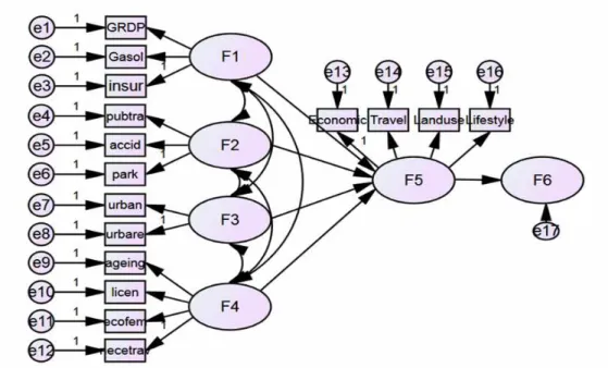
The path diagram based on research hypothesis previously set is shown in figure 8. In the diagram, the two-way arrows represent the correlation between exogenous latent variables, but do not mean that causality clearly exists. In the model, this study has set the correlation among F1, F2, F3 and F4 which mean four latent variables by order (see p.34). F5 represent the synthesized importance factor. Error terms e1~e17, except e17, are measurement error of observed variables, and e17 is residual of endogenous latent variables. It means unexplained variation from latent variables. Lastly, measurement error means the extent to which the observed variables are not describing the latent variables.(Bae, 2011).

Figure 8. Path diagram for the hypothetical model

(55)

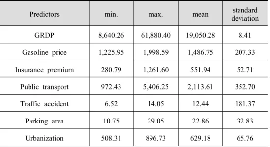
Predictors min. max. mean standard deviation

GRDP 8,640.26 61,880.40 19,050.28 8.41

Gasoline price 1,225.95 1,998.59 1,486.75 207.33

Insurance premium 280.79 1,261.60 551.94 52.71

Public transport 972.43 5,406.25 2,113.61 352.70

Traffic accident 6.52 14.05 12.44 181.37

Parking area 10.75 29.05 22.86 32.83

Urbanization 508.31 896.73 629.18 65.76

Table 4. The descriptive statistics of economic factors