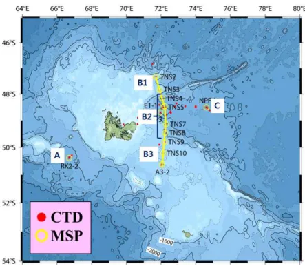
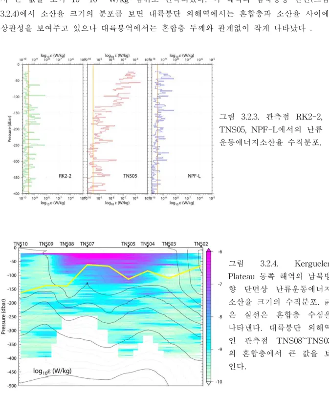
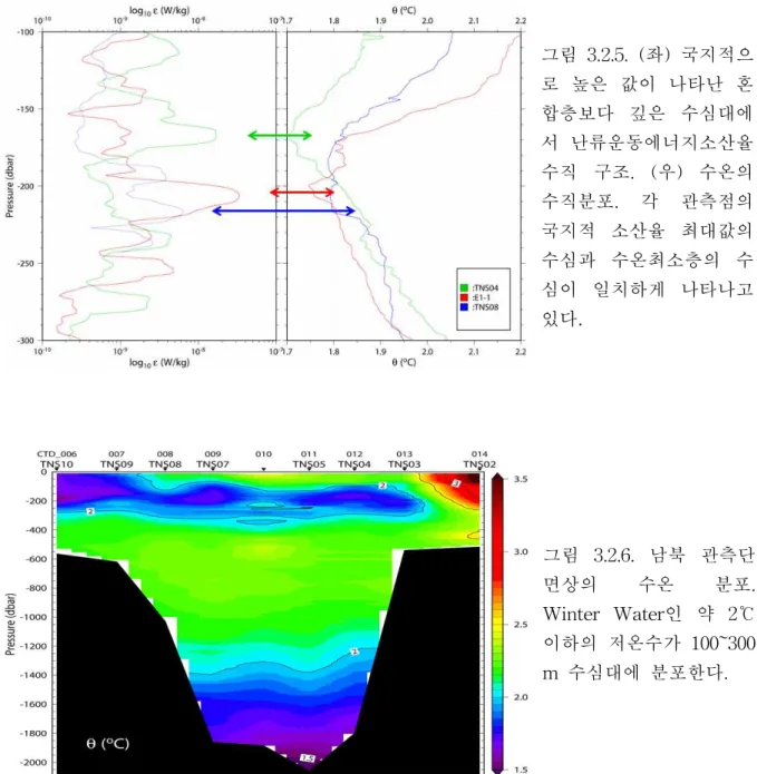
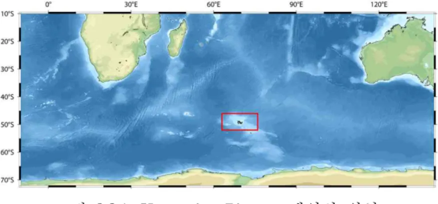
한글 난류 수직확산계수, 난류운동에너지소산율, 난류, 남극해, 공동연구. 극 방향 열 플럭스 조사를 위한 합동 Udintsev 골절 구역 관찰 프로젝트. 케르겔렌 고원 주변 관측자료 교환(CTD, LADCP, SADCP 자료 획득) - 난류확산계수 처리 방향에 대한 논의.
Kerguelen Plateau 주변의 CTD 데이터에서 난류 확산 계수 계산.
Validation of the Thorpe scale-derived vertical diffusivities against microstructure measurements in the Kerguelen region
Introduction
Validation of vertical diffusivity obtained on the Thorpe scale against microstructure measurements in the Kerguelen region. The aim of this study is to estimate vertical diffusivities from fine-scale rock density profiles using the Thorpe scale method and validate them against microstructure measurements collected via TurboMAP during the KEOPS2 cruise. It is known that the performance of the Thorpe scale method compared to microstructure estimates depends on the stratification of the water column and the conditions of the surface environment that affect the motion of the ship.
Although good agreement between the two methods has been reported in low latitude regions with high stratification and low wind (Ferron et al., 1998; Klymak et al., 2008), the application of the Thorpe scaling method in the Southern Ocean may be compromised due to low stratification and extreme environments (Frants et al., 2013). On the other hand, Shih et al. 2005) recently proposed a new parameter setting for the energetic turbulence regime (e/nN2 >) based on laboratory and numerical experiments. Note that for the moderate turbulence intensity regime (7 < e/nN2 < 100), the parameterization of K Shih et al.
Due to their extreme importance, the detailed procedures for the preliminary processing of the CTD data as well as for the detection and validation of overturns for the calculation of the Thorpe scale are given in Section 2. We will show in Section 3 that the results are sensitive to choice of K-parameterization and to the criteria for the rollover validation. In section 4, we present vertical diffusivities in the KEOPS2 area estimated from the optimally chosen parameterization and overturning ratio.
Preliminary processing of CTD data
These two (direct and indirect) estimates of e can be applied to the above two parameterizations of K, yielding a total of four types of estimates at each station of intercomparison. We tracked segments of print outlines and pointed out the data between successive encounters of the same print, although this can also be done via the data processing module “Loop Edit”. To further reduce any point-like deviations in property profiles (salinity, potential temperature, potential density), we applied a quadratic fit to consecutive 10-m segments to detect and discard "extremely anomalous" deviations greater than 4 times the root mean squared exceedance (rms) anomaly relative to the fitting curve.
To do this, we averaged the property profiles over a 10 cm window centered at each depth by a regular span of 10 cm. On average, about 2-3 scans go into this 10-cm averaging, which roughly corresponds to an average fall rate of . Also note that most density profiles start from 20 m below the sea surface, because the measurements near the surface of the ten have shown that they are highly contaminated, probably due to turbulence generated by the hull.
Thorpe scale analysis
On the other hand, a classic measure of tilt length is the Ozmidov scale LO. A similar profile is also created, starting from bottom to top, and a final intermediate profile used here is the average of the two individual (down and up) profiles. In this case, the corresponding diffusivity is set to 10-5m2s-1, a value close to the minimum of the TurboMAP-derived diffusivity in our study area.
We also show in the same figure KO_T and KS_T estimated using the Ro=0.2 criterion, always compared to KO_E and KS_E (Fig.4b). To statistically evaluate the sensitivity of vertical diffusivity to its parameterization, we calculated for all stations and intercomparison depths the ratio of diffusivities obtained from the Thorpe scale and diffusivities derived from TurboMAP, separately using the Osborn parameterization (KO_T/KO_E) and the parameter See (KS_T/KS_E) (Fig.5). This is probably due to a very low stratification of the surface mixed layer, which prevents the detection of moderate inversions whose density changes are smaller than our threshold noise level of 7x10⁻⁴ kgm-3 .
With the Osborn parameterization (Fig.5c), the Thorpe scale-derived diffusivities below 200 m overestimate (compared to the TurboMAP-derived diffusivities) with an average Rdif of ~4, with a (± 1st) variability of average. In contrast, the Shih parameterization (Fig.5d) yields a very reasonable agreement, with an average Rdif close to unity (0.3, 3) over most of the water column, except that the surface layer always has a general but somewhat tone reduced tendency to underestimate by. Consequently, we conclude that the use of the Shih parameterization, rather than the Osborn parameterization, is highly desirable in the estimation of vertical diffusivities.
Thorpe scale-derived vertical diffusivities in the KEOPS 2 area
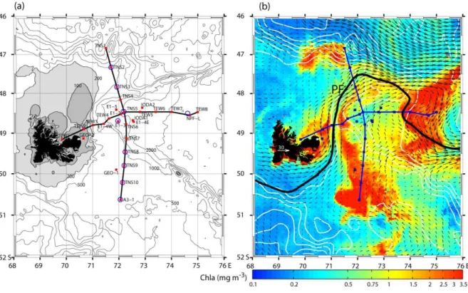
There is a clear tendency to overestimate the Osborn parameterization, especially in the layer deeper than 100 m by up to two orders of magnitude or more (Fig.5a). This is much less apparent with the Shih parameterization, which shows a relatively very compact variability of the ratio within an order of magnitude around unity (Fig. 5b). For example, in the N-S transect (Fig. 6a), the areas of elevated diffusivities are mostly confined in the seasonal thermocline (<150 m) above the winter water core developed south of the polar front, with the exception of the continental slope east of the Kerguelen Islands (Sts. TNS7-9), where the diffusion rate is low.
The strongest diffusivities are found over the shallow plateau (~600 m) southeast of the islands (St. TNS10 and A3-1) and near the PF over the northern escarpment northeast of the islands (St. Note that most of these diffusivity stations of elevated are associated with a local patch of high chlorophyll or its downstream extension, except in TNS5 where a local chlorophyll minimum is observed instead (see Fig. 1b). On the other hand, the winter water layer (150-250 m) generally coincides with the layer of minimum diffusivity.
In the Subantarctic waters north of the Polar Front (St. TNS1-2), in contrast, the diffusion rate is quite low along the upper 400 m, staying close to the background level of O (10-5m2s-1). In the E-W transect (Fig. 6b), the spatial distribution of K is quite complex compared to the N-S section and no simple pattern appears that can be easily related to the frontal circulation of water masses. However, we observe a relatively strong O diffusion rate (10-4m2s-1) over most of the water column in E1-4W located near the northward flowing PF along the escarpment east of the Kerguelen Islands, while the weakest rate of O(10-5m2s-1) is observed in TEW7 where an apparent southward intrusion of relatively warm Subantarctic surface water is associated with southward reflecting PF (see Fig.1b).
Concluding remark
The comparative results appear to be sensitive to the choice of diffusivity parameterization and tilt validation criteria. The use of the Shih parameterization (Eq. 2 and 5) in combination with a new tilting criterion of Ro = 0.25 has yielded much better results by a factor of 5 compared to the results obtained with the Osborn parameterization (Eq. 1 and 6) and the Ro = 0.2 criterion (Gargett and Garner, 2008). This study demonstrates that the Thorpe scaling method is still a useful tool for studying fine-scale diffusivity in the upper ocean, if one judiciously uses the combined Shih parameterization and the Ro = 0.25- criterion.
The latter feature is particularly pronounced at stations over the shallow plateau southeast of the Kerguelen Islands and in the cold side of the PF that runs along the escarpment northeast of the islands. On the other hand, at stations directly north of the PF where warmer Subantarctic surface water is encountered, diffusivity values are particularly low. Ratio profiles of the Thorpe scale-derived diffusivities and the TurboMAP-derived diffusivities at all intercomparison stations based on (a) the Osborn parameterization and (b) the Shih parameterization.
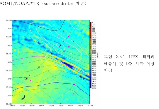
(a) N-S 횡단면 및 (b) E-W 횡단면(상단 패널, 그림 1 참조)에서 상위 400m의 소프 스케일 파생 확산 섹션(Shih 매개변수화 및 Ro = 0.25 기준을 사용하여 계산) 횡단 및 역의 위치). 수괴의 3D 전면 순환과 함께 쉽게 해석할 수 있도록(그림 1 참조) 해당 온도 섹션(중간 패널)과 해저 프로필(하단 패널)도 표시됩니다. 제3절 남극해 Udintsev 골절대 공동관측계획1). 극열 플럭스 메커니즘: 장기 해양 기후 관점에서 남극해의 평균 수온 분포는 변화 없이 평형을 이룹니다.
그러나 남극순환해류를 통과하는 해역의 상층부에는 바람장의 특성상 적도 열유속이 있으므로 이를 상쇄하는 극방향 열유속이 있어야 한다. 약 10Sv가 태평양으로 흘러 UFZ에서의 수송량을 계산할 수 있다면 태평양(동해와 서해)에서 남극 순환수류의 흐름 유형에 대한 기초자료가 된다.
이 보고서는 미래창조과학부에서 시행한 국제협력기반조성사업의 연 구보고서입니다