Copyright © The Institute of Positioning, Navigation, and Timing http://www.ipnt.or.kr Print ISSN: 2288-8187 Online ISSN: 2289-0866
1. IntroductIon
Responding to the increasing need for high-precision localization across numerous markets, high-precision positioning technologies based on Global Navigation Satellite System (GNSS) are being developed and implemented.
Unmanned vehicles including self-driving automobiles and
Evaluation of Single-Frequency Precise Point Positioning Performance Based on SPARTN Corrections Provided by the SAPCORDA SAPA Service
Yeong-Guk Kim
1,2, Hye-In Kim
2†, Hae-Chang Lee
1, Miso Kim
2, Kwan-Dong Park
1,21
Department of Geoinformatic Engineering, Inha University, Incheon 22212, Korea
2
PP-Solution Inc., Seoul 08504, Korea
ABStrAct
Fields of high-precision positioning applications are growing fast across the mass market worldwide. Accordingly, the industry is focusing on developing methods of applying State-Space Representation (SSR) corrections on low-cost GNSS receivers.
Among SSR correction types, this paper analyzes Safe Position Augmentation for Real Time Navigation (SPARTN) messages being offered by the SAfe and Precise CORrection DAta (SAPCORDA) company and validates positioning algorithms based on them. The first part of this paper introduces the SPARTN format in detail. Then, procedures on how to apply Basic-Precision Atmosphere Correction (BPAC) and High-Precision Atmosphere Correction (HPAC) messages are described. BPAC and HPAC messages are used for correcting satellite clock errors, satellite orbit errors, satellite signal biases and also ionospheric and tropospheric delays. Accuracies of positioning algorithms utilizing SPARTN messages were validated with two types of positioning strategies: Code-PPP using GPS pseudorange measurements and PPP-RTK including carrier phase measurements.
In these performance checkups, only single-frequency measurements have been used and integer ambiguities were estimated as float numbers instead of fixed integers. The result shows that, with BPAC and HPAC corrections, the horizontal accuracy is 46% and 63% higher, respectively, compared to that obtained without application of SPARTN corrections. Also, the average horizontal and vertical RMSE values with HPAC are 17 cm and 27 cm, respectively.
Keywords: SSR, SPARTN, SAPCORDA, PPP-RTK, code-PPP
drones, known as the key technology of the Fourth Industrial Revolution, is one of the growing markets. The general public is also using more Location Based Service (LBS) applications in diverse parts of daily life. Thus, the industry is focusing on high-precision GNSS researches according to the rising demand from the mass market.
There are two conditions for the mass market to fully utilize high-precision positioning. First, the correction data service, which is vital to improving positioning accuracy, should be available to a large number of users without significant barriers.
Second, the receiver price should be reasonable so that the user can easily afford it. Accordingly, the GNSS industry is seeing a growth in developing State Space Representation (SSR) corrections applied on low-cost receivers.
In SSR-based positioning, the service provider collects real-time GNSS observations from the reference network Received Feb 05, 2021 Revised Feb 24, 2021 Accepted Mar 03, 2021
†
Corresponding Author E-mail: [email protected]
Tel: +82-2-6925-1516 Fax: +82-2-6455-4305
Yeong-Guk Kim https://orcid.org/0000-0003-4770-813X
Hye-In Kim https://orcid.org/0000-0002-3256-9037
Hae-Chang Lee https://orcid.org/0000-0002-3133-2871
Miso Kim https://orcid.org/0000-0002-6959-1991
Kwan-Dong Park https://orcid.org/0000-0003-1538-8768
https://doi.org/10.11003/JPNT.2021.10.2.75
and models each error component individually and then transmits the corresponding error information to the user.
Usually, SSR messages contain corrections for five error terms: satellite orbit error, satellite clock error, satellite signal bias, ionospheric delay, and tropospheric delay. The data transfer is more efficient than the traditional Observation Space Representation or OSR method because error corrections are separated according to each error source (Kim 2016). In addition, the number of users is unlimited because two-way communication is not necessary. Due to such features, SSR correction is recognized as a viable solution for precise positioning service aimed at handling unlimited number of users. Positioning techniques utilizing SSR corrections are SBAS, PPP, and PPP-RTK, which are distinguished according to the kind of GNSS observation and correction types used.
Although GNSS positioning based on SSR messages is acknowledged as one of the key technologies that meet the market demand for high-accuracy localization, its international standard is being made and has not been finalized. Therefore, most of the current SSR service providers choose their own proprietary format and do not open the specifics to the public. Services like CenterPoint RTX by Trimble, Seastar by Fugro, and StarFire by Navcom are some examples of un-disclosed formats. SSR transmission standards that are open, on the other hand, are Compact SSR by Japan’s QZSS (Japan Cabinet Office 2020), SSRZ by Germany’s Geo++ (Geo++ 2020), and Safe Position Augmentation for Real Time Navigation (SPARTN) by SAfe and Precise CORrection DAta (SAPCORDA).
The leading company in the affordable GNSS module and chipset market, u-blox, has created a joint venture called SAPCORDA with Bosch, Geo++, and Mitsubishi Electric in August 2017. This venture focuses on developing SSR correction service, which they named Safe And Precise Augmentation Service (SAPA). The SSR format provided through SAPA is called SPARTN (SAPCORDA 2020a). Vana et al. (2019) conducted a research on GNSS correction services for high-precision GNSS positioning suitable for automotive applications. The research focused on analyzing SPARTN messages and compared SSR and Compact SSR protocols. They found that horizontal positioning accuracy with SPARTN messages was 0.8~1.6 m for the initial 20 seconds. After reaching convergence in about 30 seconds, the horizontal accuracy improved to better than 10 cm, with Root Mean Square Error (RMSE) of 4.5 cm. However, the research paper does not provide details on data processing methods nor positioning accuracy analysis. Other than this article, we could not find any other journal publication on GNSS processing utilizing SPARTN SSR messages.
This paper introduces the SPARTN message field structure and summarizes the essential procedures of converting SPARTN messages to the range measurement error. Especially, differences between Basic-Precision Atmosphere Correction (BPAC) and High-Precision Atmosphere Correction (HPAC) are described in detail. In the second half, Code-PPP and ambiguity-float PPP-RTK positioning results obtained with single-frequency GPS measurements are analyzed.
2. oVErVIEW oF SPArtn
SAPCORDA SAPA service provides SSR corrections in SPARTN format. According to SAPA datasheet Version 1.4, SSR corrections are broadcasted through the Internet or Geostationary Satellite L-Band with a continental data rate of 2400 bps (SAPCORDA 2020b). As shown in Fig. 1, as of today, the SAPA service covers all the major European regions and the continental U.S.A and plans to broaden the target area globally. There are three types of SAPA services depending on the positioning accuracy it provides: Basic, Premium, Premium+. SAPA Basic is a service for PPP and the horizontal accuracy is 30 cm to 1 m at 2-sigma (95%). SAPA Premium and Premium+ are for PPP-RTK with an improved horizontal accuracy that is better than 10 cm at 2-sigma.
Overall, Premium and Premium+ are high-precision services that allow convergence within 10 seconds while providing horizontal accuracy of 3 cm to 6 cm. This is reachable under the conditions of using error-free GNSS observation data, receiving complete and uninterrupted SAPA correction data, and utilizing ambiguity-fixed positioning. The difference between Premium and Premium+ is that integrity messages are added in the “Premium+” service. Details of each service type is listed in Table 1.
The SPARTN standard format gets updated based on collaborations among participating companies and interoperability tests. Bosch, Geo++, Mitsubishi Electric, Septentrio, and u-blox are the partners that cooperate in this research collaboration. Details of the format are published in SPARTN Interface Control Documentation (ICD) documents.
Version 1.8 of the ICD is freely available on the web and
Fig. 1. SAPA service coverage (SAPCORDA SAPA Service 2021).
http://www.ipnt.or.kr version 2.0 is being provided upon request. The former
version includes only GPS and GLONASS corrections, while the latter added additional signals, GNSS constellations, and integrity messages (SPARTN Format 2021). Users can easily decode SPARTN messages following the definitions described in the ICD document.
3. SPArtn corrEctIon
3.1 SPARTN Messages
Each SPARTN message frame has five sections as shown in Fig. 2, and the whole frame consists of 18 Transport-layer Field (TF): TF001 through TF018. The third section “Payload”
contains error corrections needed for positioning.
Correction messages in TF016, the Payload, consists of Types 0 through 127. Types 0 through 4 are currently in use.
Type 4 is about message encryption and authentication, so the necessary information for positioning error corrections is included in Types 0, 1, 2, and 3. The correction message types and descriptions are listed in Table 2. SPARTN correction is divided into four types: Type 0 is about satellite orbit, clock, and bias errors; Type 1 is HPAC; Type 2 is Geographic Area Definition; and Type 3 is BPAC.
3.2 GNSS Orbit, Clock, Bias
The orbit correction term бO contains radial, along- track, and cross-track components in units of meters. By transforming бO to the Earth-Centered Earth-Fixed (ECEF) frame using Eq. (1), one can obtain бX. Then, as shown in Eq.
(2), by subtracting бX from the broadcast satellite position X
b, one can calculate the corrected satellite position X
orb. In Eq.
(1), e
i(i = radial, along, cross) is the direction unit vector.
бX=[e
radiale
alonge
cross]∙ δO (1)
X
orb=X
b-δX (2)
The clock correction δC is also provided in the unit of meter. Following the formula shown in Eq. (3), the corrected satellite clock t
scan be calculated by combining δC with broadcast satellite clock t
b. The term c in Eq. (3) is the speed of light constant.
- 4 - 3.2 GNSS Orbit, Clock, Bias
The orbit correction term contains radial, along-track, and cross-track components in units of meters. By transforming to the Earth-Centered Earth-Fixed (ECEF) frame using Eq.
(1), one can obtain . Then, as shown in Eq. (2), by subtracting from the broadcast satellite position , one can calculate the corrected satellite position
. In Eq. (1), (i = radial, along, cross) is the direction unit vector.
[
] (1)
(2) The clock correction is also provided in the unit of meter. Following the formula shown in Eq. (3), the corrected satellite clock can be calculated by combining with broadcast satellite clock . The term in Eq. (3) is the speed of light constant.
(3) The magnitude of satellite bias correction is available in the unit of meter. Bias correction can be simply done by subtracting the corresponding bias term from the pseudorange and carrier phase measurements. The pseudorange and carrier phase measurement types defined in SPARTN version 1.8 are C1C, C2W, C2L, L1C, L2W, L2L for GPS, and C1C, C2C, L1C, L2C for GLONASS.
3.3 HPAC and BPAC
SPARTN provides ionospheric and tropospheric delay corrections through messages Type 1 HPAC and Type 3 BPAC, respectively. Differences between BPAC and HPAC are listed in Table 3. BPAC provides the ionospheric delay correction in units of Vertical Total Electron Content (VTEC) and does not include tropospheric delay corrections. On the other hand, HPAC contains tropospheric delay corrections and one should note that the ionospheric delay correction is provided as Slant TEC (STEC) instead of VTEC.
The slant ionospheric delay in the unit of meter is computed by using HPAC polynomial coefficients and grid residuals as in Eqs. (4) and (5).
in Eq. (4) is the slant ionospheric delay of satellite , for the carrier phase measurement.
in Eq. (5) is slant ionospheric delay of satellite , for the pseudorange measurement. in Eqs. (4) and (5) is slant ionospheric delay evaluated for the polynomial for satellite , whereas is the interpolated residual slant ionosphere delay obtained from the gridded residuals. The unit for and in Eqs. (4) and (5) is TECU. A bi-linear grid interpolation is used to get , which is the residual slant delay for the requested user position. The slant ionospheric delay is computed using the distance between the user location and the area centroid in addition to the polynomial coefficient provided. More details can be found in SPARTN ICD.
(4) (3)
The magnitude of satellite bias correction is available in the unit of meter. Bias correction can be simply done by subtracting the corresponding bias term from the pseudorange and carrier phase measurements. The Fig. 2. Message frame layout (SAPCORDA 2020a).
Table 1. Key features of SAPA service (SAPCORDA SAPA Service 2021).
Grade SAPA basic SAPA premium SAPA premium+
Accuracy Coverage Data format Type of stream Integrity e.g
10 cm ~ 1 m Europe, USA SPARTN Broadcast N/A Mobile / IoT
~ 10 cm Europe, USA SPARTN Broadcast N/A
Logistics or mobile / IoT
~ 10 cm Europe, USA SPARTN Broadcast Included
Automotive / New mobility, Autonomous airborne systems
Table 2. SPARTN correction message types and descriptions (SAPCORDA 2020a).
Type Subtype Message name Description
0 0
1 2 to 15
GPS OCB GLONASS OCB TBD
GNSS orbit, clock, bias
1 0
1 2 to 15
GPS HPAC GLONASS HPAC TBD
High-precision atmosphere correction
2 0
1 to 15 GAD
TBD Geographic area definition
3 0
1 to 15
BPAC polynomial
TBD Basic-precision atmosphere correction
4
0 1 2 to 15
Dynamic key message Group authentication message
TBD Encryption and authentication support
5 to 127 TBD TBD TBD
https://doi.org/10.11003/JPNT.2021.10.2.75
pseudorange and carrier phase measurement types defined in SPARTN version 1.8 are C1C, C2W, C2L, L1C, L2W, L2L for GPS, and C1C, C2C, L1C, L2C for GLONASS.
3.3 HPAC and BPAC
SPARTN provides ionospheric and tropospheric delay corrections through messages Type 1 HPAC and Type 3 BPAC, respectively. Differences between BPAC and HPAC are listed in Table 3. BPAC provides the ionospheric delay correction in units of Vertical Total Electron Content (VTEC) and does not include tropospheric delay corrections. On the other hand, HPAC contains tropospheric delay corrections and one should note that the ionospheric delay correction is provided as Slant TEC (STEC) instead of VTEC.
The slant ionospheric delay in the unit of meter is computed by using HPAC polynomial coefficients and grid residuals as in Eqs. (4) and (5). δI
CPiin Eq. (4) is the slant ionospheric delay of satellite i, for the carrier phase measurement. δI
PRiin Eq. (5) is slant ionospheric delay of satellite i, for the pseudorange measurement. I
Piin Eqs.
(4) and (5) is slant ionospheric delay evaluated for the polynomial for satellite i, whereas I
Giis the interpolated residual slant ionosphere delay obtained from the gridded residuals. The unit for I
Piand I
Giin Eqs. (4) and (5) is TECU.
A bi-linear grid interpolation is used to get I
Gi, which is the residual slant delay for the requested user position. The slant ionospheric delay I
Piis computed using the distance between the user location and the area centroid in addition to the polynomial coefficient provided. More details can be found in SPARTN ICD.
- 4 - 3.2 GNSS Orbit, Clock, Bias
The orbit correction term contains radial, along-track, and cross-track components in units of meters. By transforming to the Earth-Centered Earth-Fixed (ECEF) frame using Eq.
(1), one can obtain . Then, as shown in Eq. (2), by subtracting from the broadcast satellite position , one can calculate the corrected satellite position
. In Eq. (1), (i = radial, along, cross) is the direction unit vector.
[
] (1)
(2) The clock correction is also provided in the unit of meter. Following the formula shown in Eq. (3), the corrected satellite clock can be calculated by combining with broadcast satellite clock . The term in Eq. (3) is the speed of light constant.
(3) The magnitude of satellite bias correction is available in the unit of meter. Bias correction can be simply done by subtracting the corresponding bias term from the pseudorange and carrier phase measurements. The pseudorange and carrier phase measurement types defined in SPARTN version 1.8 are C1C, C2W, C2L, L1C, L2W, L2L for GPS, and C1C, C2C, L1C, L2C for GLONASS.
3.3 HPAC and BPAC
SPARTN provides ionospheric and tropospheric delay corrections through messages Type 1 HPAC and Type 3 BPAC, respectively. Differences between BPAC and HPAC are listed in Table 3. BPAC provides the ionospheric delay correction in units of Vertical Total Electron Content (VTEC) and does not include tropospheric delay corrections. On the other hand, HPAC contains tropospheric delay corrections and one should note that the ionospheric delay correction is provided as Slant TEC (STEC) instead of VTEC.
The slant ionospheric delay in the unit of meter is computed by using HPAC polynomial coefficients and grid residuals as in Eqs. (4) and (5).
in Eq. (4) is the slant ionospheric delay of satellite , for the carrier phase measurement.
in Eq. (5) is slant ionospheric delay of satellite , for the pseudorange measurement. in Eqs. (4) and (5) is slant ionospheric delay evaluated for the polynomial for satellite , whereas is the interpolated residual slant ionosphere delay obtained from the gridded residuals. The unit for and in Eqs. (4) and (5) is TECU. A bi-linear grid interpolation is used to get , which is the residual slant delay for the requested user position. The slant ionospheric delay is computed using the distance between the user location and the area centroid in addition to the polynomial coefficient provided. More details can be found in SPARTN ICD.
(4) (4)
- 5 -
(5) BPAC provides area-specific average VTEC values and grid residuals at the ionosphere shell height. In Eq. (6), is the VTEC of satellite ,
is the average VTEC within the area, and
is the VTEC residual of the specified location. Units of all VTEC values are TECU. As in Eq. (6), VTEC at each grid point is calculated by adding grid residuals to the average VTEC value. The user can compute VTEC at the ionosphere pierce point (IPP) by interpolating VTEC values from the grids close to IPP and then convert the obtained VTEC value at IPP to STEC through a mapping function. More details on interpolation and transformation are available in SPARTN ICD.
(6) Tropospheric delay corrections are available only through HPAC, not BPAC. The tropospheric delay is computed as shown in Eq. (7). ̅̅̅̅ is the average zenith hydrostatic delay for the given area referenced to the zero ellipsoidal height, is the residual troposphere zenith delay for station interpolated obtained from the polynomial expansion, in units of meters. is the residual troposphere zenith delay for station interpolated from the grid points, in units of meters. The notation is the hydrostatic mapping function for the satellite elevation angle at the ellipsoidal height of the approximate user location and
is the non- hydrostatic mapping function for the satellite elevation angle (Niell 1996). can be computed using polynomial coefficients and the distance between the user location and the area centroid. A bi-linear grid interpolation is used to calculate the residual for the requested user position.
More details can be found in SPARTN ICD .
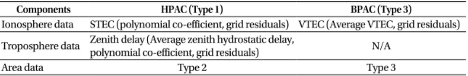
̅̅̅̅ (7) Clarification on which area and grid point the correction is about is essential in applying the ionospheric and tropospheric delay correction to the user location. Such area definition is provided through Type 2 for HPAC and Type 3 for BPAC. Fig. 3 illustrates the grid layout of the area data, and BPAC and HPAC share the same structure. The area data includes “Area ID”
which shows the area the correction refers to. The Area Reference Point (ARP) is defined to establish the grid layout. The grid node count and spacing for both longitude and latitude are provided with regards to the ARP coordinate. Among the green grid nodes, the first or upper left dot corresponds to ARP. The red dot is the polynomial expansion point which is used for calculation of the ionospheric and tropospheric delay based on HPAC polynomial coefficients.
4. POSITIONING ACCURACY ASSESSMENT WITH SPARTN
In this section, the positioning accuracy of SPARTN SSR correction was validated. We developed GPS Code-PPP and PPP-RTK post-processing algorithms based on single-frequency using the MATLAB software. While Code-PPP uses pseudorange measurements only, PPP-RTK processes pseudoranges and carrier phases together. Also, the PPP-RTK algorithm developed uses float ambiguity solutions, not fixed ones. The SPARTN SSR message utilized was broadcasted in Europe on Day of Year (DOY) 148 of year 2020 and this data was provided by
(5)
BPAC provides area-specific average VTEC values and grid residuals at the ionosphere shell height. In Eq. (6), VTEC
iis the VTEC of satellite i, VTEC
Avgis the average VTEC within the area, and VTEC
Gridis the VTEC residual of the specified location. Units of all VTEC values are TECU. As in Eq. (6), VTEC at each grid point is calculated by adding grid residuals to the average VTEC value. The user can compute
VTEC at the ionosphere pierce point (IPP) by interpolating VTEC values from the grids close to IPP and then convert the obtained VTEC value at IPP to STEC through a mapping function. More details on interpolation and transformation are available in SPARTN ICD.
VTEC
i= VTEC
Avg+ VTEC
Grid(6)
Tropospheric delay corrections are available only through HPAC, not BPAC. The tropospheric delay is computed as shown in Eq. (7).
- 5 -
(5) BPAC provides area-specific average VTEC values and grid residuals at the ionosphere shell height. In Eq. (6), is the VTEC of satellite ,
is the average VTEC within the area, and
is the VTEC residual of the specified location. Units of all VTEC values are TECU. As in Eq. (6), VTEC at each grid point is calculated by adding grid residuals to the average VTEC value. The user can compute VTEC at the ionosphere pierce point (IPP) by interpolating VTEC values from the grids close to IPP and then convert the obtained VTEC value at IPP to STEC through a mapping function. More details on interpolation and transformation are available in SPARTN ICD.
(6) Tropospheric delay corrections are available only through HPAC, not BPAC. The tropospheric delay is computed as shown in Eq. (7). ̅̅̅̅ is the average zenith hydrostatic delay for the given area referenced to the zero ellipsoidal height, is the residual troposphere zenith delay for station interpolated obtained from the polynomial expansion, in units of meters. is the residual troposphere zenith delay for station interpolated from the grid points, in units of meters. The notation is the hydrostatic mapping function for the satellite elevation angle at the ellipsoidal height of the approximate user location and
is the non- hydrostatic mapping function for the satellite elevation angle (Niell 1996). can be computed using polynomial coefficients and the distance between the user location and the area centroid. A bi-linear grid interpolation is used to calculate the residual for the requested user position.
More details can be found in SPARTN ICD .
̅̅̅̅
(7) Clarification on which area and grid point the correction is about is essential in applying the ionospheric and tropospheric delay correction to the user location. Such area definition is provided through Type 2 for HPAC and Type 3 for BPAC. Fig. 3 illustrates the grid layout of the area data, and BPAC and HPAC share the same structure. The area data includes “Area ID”
which shows the area the correction refers to. The Area Reference Point (ARP) is defined to establish the grid layout. The grid node count and spacing for both longitude and latitude are provided with regards to the ARP coordinate. Among the green grid nodes, the first or upper left dot corresponds to ARP. The red dot is the polynomial expansion point which is used for calculation of the ionospheric and tropospheric delay based on HPAC polynomial coefficients.
4. POSITIONING ACCURACY ASSESSMENT WITH SPARTN
In this section, the positioning accuracy of SPARTN SSR correction was validated. We developed GPS Code-PPP and PPP-RTK post-processing algorithms based on single-frequency using the MATLAB software. While Code-PPP uses pseudorange measurements only, PPP-RTK processes pseudoranges and carrier phases together. Also, the PPP-RTK algorithm developed uses float ambiguity solutions, not fixed ones. The SPARTN SSR message utilized was broadcasted in Europe on Day of Year (DOY) 148 of year 2020 and this data was provided by
is the average zenith hydrostatic delay for the given area referenced to the zero ellipsoidal height, T
Pis the residual troposphere zenith delay for station interpolated obtained from the polynomial expansion, in units of meters. T
Gis the residual troposphere zenith delay for station interpolated from the grid points, in units of meters.
The notation m
h(є
i,h) is the hydrostatic mapping function for the satellite elevation angle є
iat the ellipsoidal height h of the approximate user location and m
nh(є
i) is the non-hydrostatic mapping function for the satellite elevation angle (Niell 1996). T
Pcan be computed using polynomial coefficients and the distance between the user location and the area centroid.
A bi-linear grid interpolation is used to calculate the residual T
Gfor the requested user position. More details can be found in SPARTN ICD.
- 5 -
(5) BPAC provides area-specific average VTEC values and grid residuals at the ionosphere shell height. In Eq. (6), is the VTEC of satellite ,
is the average VTEC within the area, and
is the VTEC residual of the specified location. Units of all VTEC values are TECU. As in Eq. (6), VTEC at each grid point is calculated by adding grid residuals to the average VTEC value. The user can compute VTEC at the ionosphere pierce point (IPP) by interpolating VTEC values from the grids close to IPP and then convert the obtained VTEC value at IPP to STEC through a mapping function. More details on interpolation and transformation are available in SPARTN ICD.
(6) Tropospheric delay corrections are available only through HPAC, not BPAC. The tropospheric delay is computed as shown in Eq. (7). ̅̅̅̅ is the average zenith hydrostatic delay for the given area referenced to the zero ellipsoidal height, is the residual troposphere zenith delay for station interpolated obtained from the polynomial expansion, in units of meters. is the residual troposphere zenith delay for station interpolated from the grid points, in units of meters. The notation is the hydrostatic mapping function for the satellite elevation angle at the ellipsoidal height of the approximate user location and
is the non- hydrostatic mapping function for the satellite elevation angle (Niell 1996). can be computed using polynomial coefficients and the distance between the user location and the area centroid. A bi-linear grid interpolation is used to calculate the residual for the requested user position.
More details can be found in SPARTN ICD .
̅̅̅̅
(7) Clarification on which area and grid point the correction is about is essential in applying the ionospheric and tropospheric delay correction to the user location. Such area definition is provided through Type 2 for HPAC and Type 3 for BPAC. Fig. 3 illustrates the grid layout of the area data, and BPAC and HPAC share the same structure. The area data includes “Area ID”
which shows the area the correction refers to. The Area Reference Point (ARP) is defined to establish the grid layout. The grid node count and spacing for both longitude and latitude are provided with regards to the ARP coordinate. Among the green grid nodes, the first or upper left dot corresponds to ARP. The red dot is the polynomial expansion point which is used for calculation of the ionospheric and tropospheric delay based on HPAC polynomial coefficients.
4. POSITIONING ACCURACY ASSESSMENT WITH SPARTN
In this section, the positioning accuracy of SPARTN SSR correction was validated. We developed GPS Code-PPP and PPP-RTK post-processing algorithms based on single-frequency using the MATLAB software. While Code-PPP uses pseudorange measurements only, PPP-RTK processes pseudoranges and carrier phases together. Also, the PPP-RTK algorithm developed uses float ambiguity solutions, not fixed ones. The SPARTN SSR message utilized was broadcasted in Europe on Day of Year (DOY) 148 of year 2020 and this data was provided by
(7)
Clarification on which area and grid point the correction is about is essential in applying the ionospheric and tropospheric delay correction to the user location. Such area definition is provided through Type 2 for HPAC and Type 3 for BPAC. Fig. 3 illustrates the grid layout of the area data, and BPAC and HPAC share the same structure. The area data includes “Area ID” which shows the area the correction refers to. The Area Reference Point (ARP) is defined to establish the grid layout. The grid node count and spacing for both longitude and latitude are provided with regards to the ARP coordinate. Among the green grid nodes, the first or upper left dot corresponds to ARP. The red dot is the polynomial expansion point which is used for calculation of the ionospheric and tropospheric delay based on HPAC polynomial coefficients.
Table 3. Comparison of HPAC and BPAC messages.
Components HPAC (Type 1) BPAC (Type 3)
Ionosphere data STEC (polynomial co-efficient, grid residuals) VTEC (Average VTEC, grid residuals) Troposphere data Zenith delay (Average zenith hydrostatic delay,
polynomial co-efficient, grid residuals) N/A
Area data Type 2 Type 3
http://www.ipnt.or.kr
4. PoSItIonInG AccurAcY ASSESSMEnt WItH SPArtn
In this section, the positioning accuracy of SPARTN SSR correction was validated. We developed GPS Code-PPP and PPP-RTK post-processing algorithms based on single- frequency using the MATLAB software. While Code-PPP uses pseudorange measurements only, PPP-RTK processes pseudoranges and carrier phases together. Also, the PPP-RTK algorithm developed uses float ambiguity solutions, not fixed ones. The SPARTN SSR message utilized was broadcasted in Europe on Day of Year (DOY) 148 of year 2020 and this data was provided by SAPCORDA. The GPS data is 1-second interval measurements collected by the SCDE reference station on the same day. The SCDE reference station is located in Germany as seen in Fig. 4.
4.1 Code-PPP
In Code-PPP positioning, SSR corrections were combined with GPS single-frequency pseudorange observations. The site coordinate was computed at every second with least- squares estimation (LSE). The first 20-minute measurements at every hour were taken on DOY 148 of year 2020. Thus 24 datasets were tested to analyze the positioning accuracy. We compared results of three positioning scenarios: 1) without SSR corrections, 2) with BPAC corrections, and 3) with HPAC corrections. In this paper we denote each scenario as ‘SPP’,
‘BPAC’, and ‘HPAC’ for brevity. SPP stands for Standard Point Positioning, and BPAC and HPAC correspond to SPARTN correction types described in Section 3.
Eq. (8) is the Code-PPP pseudorange measurement equation between receiver r and satellite i. In the equation, p
riis the pseudorange measurement, ρ
riis the 3D distance between the receiver and the satellite, c is the speed of light, δt
ris the receiver clock offset, δt
iis the satellite clock offset, I
riis ionospheric delay, T
riis tropospheric delay, B
piis satellite code bias error, M
riis multipath error, and ε
pis pseudorange
measurement noise.
- 6 -
SAPCORDA. The GPS data is 1-second interval measurements collected by the SCDE reference station on the same day. The SCDE reference station is located in Germany as seen in Fig. 4.
4.1 CODE-PPP
In Code-PPP positioning, SSR corrections were combined with GPS single-frequency pseudorange observations. The site coordinate was computed at every second with least-squares estimation (LSE). The first 20-minute measurements at every hour were taken on DOY 148 of year 2020. Thus 24 datasets were tested to analyze the positioning accuracy. We compared results of three positioning scenarios: 1) without SSR corrections, 2) with BPAC corrections, and 3) with HPAC corrections. In this paper we denote each scenario as „SPP‟, „BPAC‟, and „HPAC‟
for brevity. SPP stands for Standard Point Positioning, and BPAC and HPAC correspond to SPARTN correction types described in Section 3.
Eq. (8) is the Code-PPP pseudorange measurement equation between receiver and satellite . In the equation, is the pseudorange measurement, is the 3D distance between the receiver and the satellite, is the speed of light, is the receiver clock offset, is the satellite clock offset, is ionospheric delay, is tropospheric delay, is satellite code bias error, is multipath error, and is pseudorange measurement noise.
( ) (8) Eq. (9) is the state vector for the Code-PPP estimation algorithm, and ( ) are the coordinates of the receiver.
(9) In the case of SPP, orbit-clock-bias errors were not corrected for. Meanwhile, the tropospheric and ionosphere delay was accounted by Global Pressure and Temperature (GPT) by Boehm et al. (2007) and Klobuchar (1987) models, respectively. In the case of BPAC and HPAC, satellite orbit-clock-bias errors are corrected. Also, the ionospheric correction from BPAC and HPAC corrects the ionospheric delay. BPAC uses GPT to correct tropospheric delay and HPAC uses the tropospheric correction within HPAC. Error corrections and the corresponding models used for Code-PPP are listed in Table 4.
As the reference or true coordinate, we utilized the precise coordinates obtained from the web-based Automated Precision Positioning Service (APPS). The daily, 24-hour RINEX file obtained at the SCDE station on DOY 148 was uploaded to the APPS site to get the reference coordinate. The elevation cut-off angle was set to 12.5˚ in all three positioning modes. In the BPAC and HPAC processing, only those satellites whose SPARTN corrections are available were used. However, in the SPP model, all visible satellites were included in the data processing.
Fig. 5 shows Code-PPP horizontal errors processed from 12:00 to 12:20 among the 24 data sets: SPP is in red, BPAC in green, and HPAC in blue. SPP accuracy is the poorest and HPAC accuracy is better than that of BPAC. The minimum, maximum, and average of every 24 RMSE of each scenario is listed in Table 5. The average horizontal RMS error is 1.25 m for SPP, 0.86 m for BPAC, and 0.34 m for HPAC. The average vertical RMS error also improves to 2.30 m, 1.14 m, and 0.50 m.
(8)
Eq. (9) is the state vector for the Code-PPP estimation algorithm, and (x
r, y
r, z
r) are the coordinates of the receiver.
x = [x
r, y
r, z
r, δt
r] (9)
In the case of SPP, orbit-clock-bias errors were not corrected for. Meanwhile, the tropospheric and ionosphere delay was accounted by Global Pressure and Temperature (GPT) by Boehm et al. (2007) and Klobuchar (1987) models, respectively. In the case of BPAC and HPAC, satellite orbit- clock-bias errors are corrected. Also, the ionospheric correction from BPAC and HPAC corrects the ionospheric delay. BPAC uses GPT to correct tropospheric delay and HPAC uses the tropospheric correction within HPAC. Error corrections and the corresponding models used for Code- PPP are listed in Table 4.
As the reference or true coordinate, we utilized the precise coordinates obtained from the web-based Automated Precision Positioning Service (APPS). The daily, 24-hour RINEX file obtained at the SCDE station on DOY 148 was uploaded to the APPS site to get the reference coordinate.
The elevation cut-off angle was set to 12.5˚ in all three positioning modes. In the BPAC and HPAC processing, only those satellites whose SPARTN corrections are available were used. However, in the SPP model, all visible satellites were included in the data processing.
Fig. 5 shows Code-PPP horizontal errors processed from 12:00 to 12:20 among the 24 data sets: SPP is in red, BPAC in green, and HPAC in blue. SPP accuracy is the poorest and Table 4. Error correction data and models for each Code-PPP positioning scenario.
SPP BPAC HPAC
Orbit/Clock/Bias Troposphere Ionosphere
N/A GPT Klobuchar
Orbit/Clock/Bias GPT BPAC
Orbit/Clock/Bias
HPAC
HPAC
Fig. 3. SPARTN grid layout (SAPCORDA 2020a). Fig. 4. Location of the SAPCORDA SCDE reference station.
https://doi.org/10.11003/JPNT.2021.10.2.75
HPAC accuracy is better than that of BPAC. The minimum, maximum, and average of every 24 RMSE of each scenario is listed in Table 5. The average horizontal RMS error is 1.25 m for SPP, 0.86 m for BPAC, and 0.34 m for HPAC. The average vertical RMS error also improves to 2.30 m, 1.14 m, and 0.50 m.
4.2 PPP-RTK
PPP-RTK positioning algorithm used HPAC corrections along with GPS single-frequency pseudorange and carrier phase observations. The site coordinate was estimated at every second with the Kalman Filter method. The datasets are the same as those used for Code-PPP in Section 4.1; the first 20-minute measurements at every hour were taken on DOY 148 of year 2020. Thus 24 datasets were tested to analyze the positioning accuracy. The same precise coordinates obtained from APPS were used to derive position errors. The elevation cut-off angle was set to 12.5˚.
Eq. (10) is the carrier phase measurement equation: ϕ
riis the carrier phase measurement, B
ϕiis the satellite carrier bias error, ε
ϕis the carrier phase measurement noise, λ is the wavelength, and N
riis an integer ambiguity. In this case of PPP-RTK, satellite orbit-clock-bias errors are corrected. Also,
the ionospheric and tropospheric delays are also corrected using HPAC.
- 7 - 4.2 PPP-RTK
PPP-RTK positioning algorithm used HPAC corrections along with GPS single-frequency pseudorange and carrier phase observations. The site coordinate was estimated at every second with the Kalman Filter method. The datasets are the same as those used for CODE-PPP in Section 4.1; the first 20-minute measurements at every hour were taken on DOY 148 of year 2020. Thus 24 datasets were tested to analyze the positioning accuracy. The same precise coordinates obtained from APPS were used to derive position errors. The elevation cut-off angle was set to 12.5˚.
Eq. (10) is the carrier phase measurement equation: is the carrier phase measurement, is the satellite carrier bias error, is the carrier phase measurement noise, is the wavelength, and is an integer ambiguity. In this case of PPP-RTK, satellite orbit-clock-bias errors are corrected. Also, the ionospheric and tropospheric delays are also corrected using HPAC.
( ) (10) Eq. (11) is the state vector of PPP-RTK algorithm. This paper estimates the integer ambiguity with a float solution.
(11) Fig. 6 shows PPP-RTK positioning result using HPAC corrections. In the figure, the coordinate deviations for every dataset are plotted as time-series in the north-south (North), east- west (East) and up (Vertical) directions. Table 6 categorized the statistics of all the 24 datasets.
The average horizontal and vertical values are 17 cm and 27 cm, respectively. The dataset with the minimum error showed a horizontal error of 8 cm and vertical error of 4 cm. Fig. 7 depicts RMSE histogram by 5 cm bins. In the case of the horizontal direction, 22 of the 24 datasets have errors less than 30 cm and 17 datasets show errors less than 20 cm. As for the vertical error, 19 of the 24 datasets achieved accuracies better than 30 cm.
The average horizontal accuracy 17 cm, computed in Section 4.2, is poorer compared to that stated in Vana et al. (2019) and the SAPA datasheet. This is assumed to have happened due to the difference between the ambiguity-float solution and the ambiguity-fix solution. We believe that an accuracy better than the ambiguity-float will be achievable when applying SPARTN message to the ambiguity-fixing algorithm.
Therefore, it can be concluded that precise positioning with an average of 17 cm horizontal accuracy is possible when SPARTN messages are applied to an ambiguity-float PPP-RTK algorithm, even with a single-frequency receiver.
5. CONCLUSIONS
First, the details and application procedures of SPARTN messages were introduced. We also developed and assessed Code-PPP and PPP-RTK algorithms that use SPARTN corrections.
We compared three positioning scenarios of Code-PPP: SPP, processing with BPAC and processing with HPAC. With HPAC messages, the horizontal accuracy improved by 73% with respect to that of SPP. It also improved by 31% compared to that of BPAC messages. At the
(10)
Eq. (11) is the state vector of PPP-RTK algorithm. This paper estimates the integer ambiguity with a float solution.
- 7 - 4.2 PPP-RTK
PPP-RTK positioning algorithm used HPAC corrections along with GPS single-frequency pseudorange and carrier phase observations. The site coordinate was estimated at every second with the Kalman Filter method. The datasets are the same as those used for CODE-PPP in Section 4.1; the first 20-minute measurements at every hour were taken on DOY 148 of year 2020. Thus 24 datasets were tested to analyze the positioning accuracy. The same precise coordinates obtained from APPS were used to derive position errors. The elevation cut-off angle was set to 12.5˚.
Eq. (10) is the carrier phase measurement equation: is the carrier phase measurement, is the satellite carrier bias error, is the carrier phase measurement noise, is the wavelength, and is an integer ambiguity. In this case of PPP-RTK, satellite orbit-clock-bias errors are corrected. Also, the ionospheric and tropospheric delays are also corrected using HPAC.
( ) (10) Eq. (11) is the state vector of PPP-RTK algorithm. This paper estimates the integer ambiguity with a float solution.
(11) Fig. 6 shows PPP-RTK positioning result using HPAC corrections. In the figure, the coordinate deviations for every dataset are plotted as time-series in the north-south (North), east- west (East) and up (Vertical) directions. Table 6 categorized the statistics of all the 24 datasets.
The average horizontal and vertical values are 17 cm and 27 cm, respectively. The dataset with the minimum error showed a horizontal error of 8 cm and vertical error of 4 cm. Fig. 7 depicts RMSE histogram by 5 cm bins. In the case of the horizontal direction, 22 of the 24 datasets have errors less than 30 cm and 17 datasets show errors less than 20 cm. As for the vertical error, 19 of the 24 datasets achieved accuracies better than 30 cm.
The average horizontal accuracy 17 cm, computed in Section 4.2, is poorer compared to that stated in Vana et al. (2019) and the SAPA datasheet. This is assumed to have happened due to the difference between the ambiguity-float solution and the ambiguity-fix solution. We believe that an accuracy better than the ambiguity-float will be achievable when applying SPARTN message to the ambiguity-fixing algorithm.
Therefore, it can be concluded that precise positioning with an average of 17 cm horizontal accuracy is possible when SPARTN messages are applied to an ambiguity-float PPP-RTK algorithm, even with a single-frequency receiver.
5. CONCLUSIONS
First, the details and application procedures of SPARTN messages were introduced. We also developed and assessed Code-PPP and PPP-RTK algorithms that use SPARTN corrections.
We compared three positioning scenarios of Code-PPP: SPP, processing with BPAC and processing with HPAC. With HPAC messages, the horizontal accuracy improved by 73% with respect to that of SPP. It also improved by 31% compared to that of BPAC messages. At the
(11)
Fig. 6 shows PPP-RTK positioning result using HPAC corrections. In the figure, the coordinate deviations for every dataset are plotted as time-series in the north-south (North), east-west (East) and up (Vertical) directions.
Table 6 categorized the statistics of all the 24 datasets. The average horizontal and vertical values are 17 cm and 27 cm, respectively. The dataset with the minimum error showed a horizontal error of 8 cm and vertical error of 4 cm. Fig. 7 depicts RMSE histogram by 5 cm bins. In the case of the horizontal direction, 22 of the 24 datasets have errors less than 30 cm and 17 datasets show errors less than 20 cm. As for the vertical error, 19 of the 24 datasets achieved accuracies better than 30 cm.
The average horizontal accuracy 17 cm, computed in Section 4.2, is poorer compared to that stated in Vana et al. (2019) and the SAPA datasheet. This is assumed to have happened due to the difference between the ambiguity-float solution and the ambiguity-fix solution. We believe that an accuracy better than the ambiguity-float will be achievable Fig. 5. Code-PPP horizontal accuracy comparison of each scenario on
12:00~12:20.
Fig. 6. PPP-RTK errors in the north, east, and vertical directions.
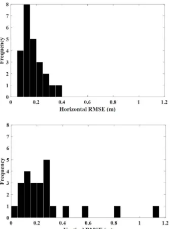
Table 5. Minimum, maximum, and average RMSE (m) from three Code-PPP positioning scenarios.
Scenario Direction Minimum Maximum Average
SPP Horizontal
Vertical 3-dimension
0.35 0.50 0.70
7.07 8.53 8.81
1.25 2.30 2.76
BPAC
Horizontal Vertical 3-dimension
0.32 0.37 0.64
4.52 6.49 7.92
0.86 1.14 1.45
HPAC Horizontal Vertical 3-dimension
0.25 0.30 0.42
0.62 0.79 0.84
0.34 0.50 0.61
Table 6. PPP-RTK minimum, maximum, and average RMSE (m).
Minimum Maximum Average