A Comparative Study on Arrhenius-Type Constitutive Models with Regression Methods

https://doi.org/10.5228/KSTP.2017.26.1.18

A Comparative Study on Arrhenius-Type Constitutive Models with Regression Methods

Kyunghoon Lee^1,# · Mohanraj Murugesan² · Seung-Min Lee¹ · Beom-Soo Kang¹ (Received October 17, 2016 / Revised December 19, 2016 / Accepted December 21, 2016)

Abstract

A comparative study was performed on strain-compensated Arrhenius-type constitutive models established with two regression methods: polynomial regression and regression Kriging. For measurements at high temperatures, experimental data of 70Cr3Mo steel were adopted from previous research. An Arrhenius-type constitutive model necessitates strain compensation for material constants to account for strain effect. To associate the material constants with strain, we first evaluated them at a set of discrete strains, then capitalized on surrogate modeling to represent the material constants as a function of strain. As a result, disparate flow stress models were formed via the two different regression methods. The constructed constitutive models were examined systematically against measured flow stresses by validation methods. The predicted material constants were found to be quite accurate compared to the actual material constants. However, notable mismatches between measured and predicted flow stresses were revealed by the proposed validation techniques, which carry out validation with not the entire, but a single tensile test case.

Keywords: Flow Stress, Arrhenius-type Constitutive Model, Polynomial Regression, Regression Kriging

1. Introduction

Understanding the flow behavior of metals and alloys at hot deformation conditions is essential in metal forming processes, such as hot rolling, forging, and extrusion[1, 2].

Many researchers have utilized constitutive equations, also known as flow stress models, to represent flow stress behavior and to investigate the response of materials under different loadings[2, 3]. For flow stress estimation at high temperature, constitutive equations can be developed based on an Arrhenius-type equation because it is applicable over a wide range of strain rates and temperatures [4].

In this paper, we exploit regression Kriging for strain compensation in the context of Arrhenius-type constitutive model construction. In addition, we compare

the utility of regression Kriging to that of polynomial regression using an experimental data set digitally extracted from the published research work[5]. For prediction quality evaluation, we apply numerical and graphical validation methods to the constructed Arrhenius-type constitutive models. In particular, we investigate the closeness of predicted and measured flow stresses of each tensile test case unlike the previous research[5], which used the whole tensile test data.

Consequently, this methodical validation shows discrepancies between the predicted and the measured flow stress, obscured in Ref.[5]. Overall, we present systematic construction and validation approaches for flow stress modeling based on the Arrhenius-type constitutive equation with regression methods.

1. Department of Aerospace Engineering, Pusan National University 2. Department of Mechanical Engineering, Sogang University

# Corresponding Author : Department of Aerospace Engineering, Pusan National University, [email protected] (Kyunghoon Lee), [email protected] (Mohanraj Murugesan), [email protected] (Beom-Soo Kang)

2. Formulations

2.1. Arrhenius-Type Constitutive Equation

The relationship between a strain rate  and a temperature T can be described with the Zener- Hollomon parameter Z [6, 7] such that

   

exp ,

Z Q RT (1)

where Q is the activation energy of deformation, and R is the gas constant, 8.314Jmol K^{1 1}. Depending on the level of flow stress, Z can be related to different flow stress expressions as follows. First, the power law equation

1 1,

Z  An (2)

where A₁ and n₁ are material constants, is commonly used for a low level of flow stress. Second, the exponential equation

2exp

 

Z A  (3) where A₂ and  are material constants, is preferred for a high level of flow stress. Last, the hyperbolic sine law equation



  

Z  A  (4)

where A, n and  are material constants, is useful for a wide range of flow stress; here  is the stress multiplier such that   n₁.

To evaluate the material constants, we first equate each of Eqs. (2) to (4) to Eq. (1) and then take log transformation, which results in

   

1 1

ln lnAn ln Q RT , (5)

   

ln  lnA2 Q RT , (6)

       

ln nln sinh  lnA Q RT . (7) After taking partial derivatives of Eqs. (5) to (7) holding T, we obtain the following equations for n₁,

, and n [5]:

   

1

ln ln ln

, , .

ln _{T T} ln sinh _T

n   n 

   

  

  

  

Similarly, by taking a partial derivative of Eq. (7) fixing

 , we can evaluate Q as follows:

   

 

ln sinh

. 1

Q nR

T _



 



For the evaluation of A₁, A₂, and A, we use the log- transform of Eqs. (2) to (4) such that

   

1 1

2

ln ln ln ,

ln ln ,

ln ln ln sinh ,

Z A n

Z A

Z A n







 

 

 

where ln A₁, ln A₂, and ln A can be found as the intercepts of straight-line equations composed of











  

 

 

   

, ; , ln , ,

ln ln

1arc sinh exp .

T Q A n

A Q RT

n

  





 

  

 

 

(8) Note that although Eq. (8) relates a temperature T and a strain rate  to flow stress  , it cannot account for strain effect; hence, strain compensation is required so that the material constants---such as Q , ln A, , and

n---can be associated with strain  as shown below:

 

 

, , ; ( ), ln ( ), ( ), ( )

ln ln ( ) ( )

1 arc sinh exp .

( ) ( )

T Q A n

A Q RT

n

       

  

  

 

   

  

  

(9) For this matter, we apply regression technology to a set of the material constants observed at strain values.

2.2. Regression Techniques 2.2.1. Polynomial regression

Polynomial regression assumes that a response of interest y_iR can be written as a p th order polynomial function of an independent variable x_iR as follows [8]:

2

0 1 2 ^p ,

i i i p i i

y  x  x   x e (10)

where

 

i R

e  is a measurement noise. For n samples of y_i observed at

 

2

1 1 1 1 1 1

2

2 2 2 2 2 2

2

1 1

,

1

p

p

p

n n n n n n

y x x x e

y x x x e

y x x x e







 

 

     

 

     

 

     

 

     

 

     

      

(11)

which can be cast as

, yXe

where yRⁿ is n observations, XR^{np1} is a design matrix, R^p1 is p1 regression coefficients, and eRⁿ is n measurement noises. The estimate of  can be evaluated as

 

ˆ X X^T X y^T ,

  ^

by the least squares method [9], [10]. Finally, the estimate of y can be found with ˆ as follows:

ˆ ˆ. yX

2.2.2. Regression Kriging

Kriging is an interpolation technique that assumes observed data are generated by a Gaussian process from a statistical perspective. Based on a Kriging formulation for interpolation, regression Kriging takes account of noise in observations. In theory, regression Kriging views an observation y x( )R, where xR^k, as a realization of a Gaussian random variable

( ) ( ) ( ),

Y x   Z x E x (12) where R is a mean trend, and both Z and E are random functions such that ^{Z ~GP}









~ 0, _ii

E GP   _ , respectively. In Eq. (12), ²R and ²R are process and noise variances, respectively,

 is a correlation function, and _ii is the Kronecker delta, whose value is 1 if ii. Note that Eq. (12) is

based on the ordinary Kriging formulation since  is constant irrespective of x. Due to the assumptions, a random vector consisting of Y is also a random function such that Y ^~GP





Gaussian distribution



 

  

N    I N    I where 1Rⁿ is a vector of n ones. Here,  ^and I are correlation matrices constructed by  and _ii, respectively, and

 is a normalized variance such that    ^{2 2. For} the evaluation of _il at an observation point





typically employed is the Gaussian correlation function

   

 

1

, exp ,

k

i l i l

j j j

j

x x x x

 



   

 





where _jR is a Kriging hyperparameter.

Since a set of observations

 

 

yy x y x  is distributed as a multivariate Gaussian, a likelihood function L is formulated for parameter estimation as follows:

 

 

2

T 1

2 1 2 2

2

; , , ,

1 1

1 exp

2 2

n . L y

y I y

I

   

  

  

    

 

 

 

 

 

(13) The estimates of  and ² can be found by the method of maximum likelihood (ML) as below:

 

 

T 1

T 1

ˆ 1 ,

1 1

I y I

 







  

 

and

  ^T  ¹ 

2 1 1

ˆ y I y .

n

  



    



After the substation of the previously obtained ˆ and ˆ2

 into Eq. (13), a concentrated log-likelihood





2 2

c

n I

        (14)

is formed and addressed by unconstrained optimization for the estimates of Kriging parameters  and . Once the ML estimates are obtained, a new observation

 ⁰

 

y  y x  at a new observation point x^{ 0} R^k can be predicted as with the derivation of parameter estimates. The log-likelihood function of y^{ 0} is found as

 

 

 

0 2

1 ˆ ˆ

( ) 1 ,

2ˆ

y y  I y 



       1 (15)

where y is augmented observations such that

 0 1

; Rⁿ

yy y  ^{ , and } and I are augmented correlation matrices such that  R^{   n  1 n1 ,}

   1 1

R^{n n}

I ^{   , namely}

T ,

1

I I 

  

    



 

 

  (16) where ^{ }_^









Finally, the prediction estimate

ˆy0 is evaluated by the method of ML such that

 ^{0 T}

  



ˆ( ) ˆ 1ˆ .

y x     I ^ y 

3. Material Constants Modeling

3.1. Experimental Data

For this comparative study, we used digitally extracted data of 70Cr3Mo steel in Ref. [5]. We removed the elastic region from the true stress-strain data to keep only the plastic stress-strain curve. The experimental cases are outlined in Table 1. For details of the stress-strain data acquisition, please see Ref. [5].

Table 1 Experimental conditions of 70Cr3Mo steel [5]

for flow stress modeling

3.2. Model Construction

As delineated in Section 2.1, the influence of strain on flow stress is not taken into account in the Arrhenius-type

Table 2 Estimated coefficients of polynomial regression models with 70Cr3Mo steel

Q (kJ/mol) ln A(s^{1) (MPa) n}

ˆ0

 3.802e2 3.267e1 1.490e2 ^6.205 ˆ1

 8.295e2 7.181e1 -5.411e2 1.829 ˆ2

 -5.833e3 -5.010e2 2.390 e1 -5.898e1 ˆ3

 1.522e4 1.284e3 -4.936 e1 1.939e2 ˆ4

 -1.853e4 -1.526e3 4.803 e1 -2.634e2 ˆ5

 8.955e3 7.195e2 -1.661 e1 1.346e2

constitutive equation in Eq. (8). Because strain has a significant effect on stress, it is imperative to include strain in flow stress evaluation. For that purpose, we express the material constants of the Arrhenius-type constitutive equation, particularly Q , ln A,  , and n, as a function of strain via polynomial regression and regression Kriging. To fit regression models, we took advantage of the curve-fitting toolbox of MATLAB [11], [12] and ooDACE [13]~[15] for polynomial regression and regression Kriging, respectively. For Kriging parameter estimation, the concentrated log-likelihood in Eq. (14) was optimized by the sequential quadratic programming within a log-transformed parameter domain bounded by 5 and 5. Here polynomial regression was adopted as a comparison target since it is used in Ref. [5], and the correlations among the four material constants were neglected for the sake of simplicity.

We first employed 5th order polynomial regression and regression Kriging for each of the four material constants of 70Cr3Mo steel. The resultant estimates of polynomial regression coefficients ˆ

i and those of regression Kriging parameters





i contributes to the variation of a material constant with respect to strain change. As for regression Kriging, unlike polynomial regression necessitating a total of six parameters, only the two parameters  and  suffice; the former is for assuming the mean trend to be constant in ordinary Temperature (K) Strain rate (s^-1)

1173 0.01

1273 0.10

1373 1.00

1473 10.0

Kriging, and the latter is for having only one independent variable, strain. This difference in the number of required parameters for regression shows that regression Kriging is more compact than polynomial regression in delineating the nonlinear behavior of material constants subject to strain variation.

Table 3 Estimated parameters of regression Kriging models with 70Cr3Mo steel

Q (kJ/mol) ln A(s^{1) }

(MPa) n

ˆ 1.5653 1.4618 9.1537 e1

9.4449 e2 ˆ2

 3.7969e2 2.9870 3.8265

e6 ^2.2276

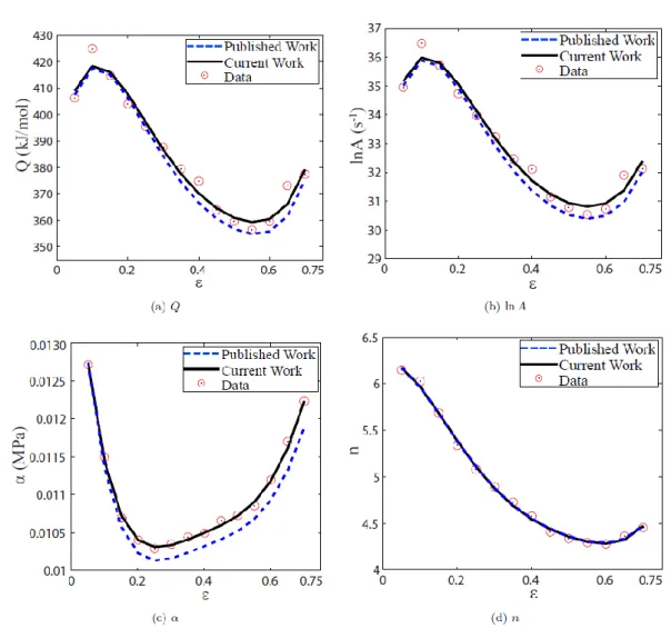
To cross-validate the estimated polynomial regression coefficients in Table 2 to those published in Ref. [5], we drew the polynomial regression functions of the material constants as shown in Fig. 1. Here, current and published refer to polynomial regression models developed by the current authors and by the previous researchers [5], and data indicates the digitally extracted data, not the genuine data. Figure 1 shows that both the current and the published polynomial regression models are quite alike, which conveys that digitization errors are inconsiderable.

Overall, we conclude that the digitally extracted data would not significantly deviate from the original data in Ref. [5].

Fig. 1 Polynomial regression models of material constants for 70Cr3Mo steel

3.3. Model Validation

For the validation of regression models for material constants, we adopted both numerical and graphical methods. For the former, we utilized numerical metrics, such as the coefficient of determination  R² , an average absolute relative error (AARE), and an absolute relative error (ARE). First, an R²value shows the degree of variation explained by a regression model and is defined by

 

 

2 2

2

ˆ

1 ^{i i i} ,

i i

y y R

y y

  



 

where y_i and yˆ_i are actual and predicted data, respectively, and y is the mean value of actual data.

Second, an ARE value denotes the magnitude of relative error of predicted data with respect to actual data and is defined by

ARE= ˆ^{i i} .

i

y y y



Third, an AARE value is the mean of AREs and is defined by

1

1 ˆ

AARE= ^{i i} ,

i N

i

y y N  y



where N is the number of predicted/actual data. Note that instead of a correlation coefficient r, we used R² because it is more appropriate to evaluate the prediction capability of a regression model than the strength of a

linear dependence between predicted and actual data.

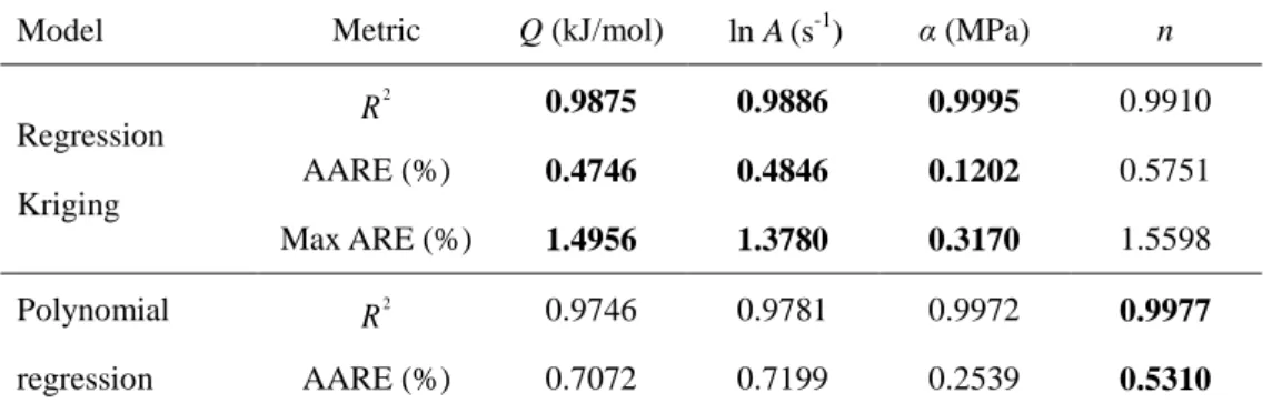
Table 4 presents the values of numerical validation metrics associated with polynomial regression and regression Kriging models. Note that a bold-faced number indicates that the corresponding surrogate outperforms the other hereinafter. In Table 4, regression Kriging demonstrates slightly more favorable values than polynomial regression; Q and n are better fitted by regression Kriging and polynomial regression, respectively. Because of acceptable numerical validation results in Table 4, the predicted material constants closely align with the observed material constants in Fig. 2.

4. Flow Stress Model Validation

As with the validation of material constants, we followed the same validation procedures to examine Arrhenius-type flow stress models based on the developed regression models. Note that unlike the previous research in Ref. [5], which validated the entire set of flow stress predictions at once, we separately

validated each set of flow stress predictions one by one.

This alternative validation scheme is rooted in the fact that one typically predicts flow stress at a specific temperature and strain rate condition, not at the whole temperature and strain rate conditions.

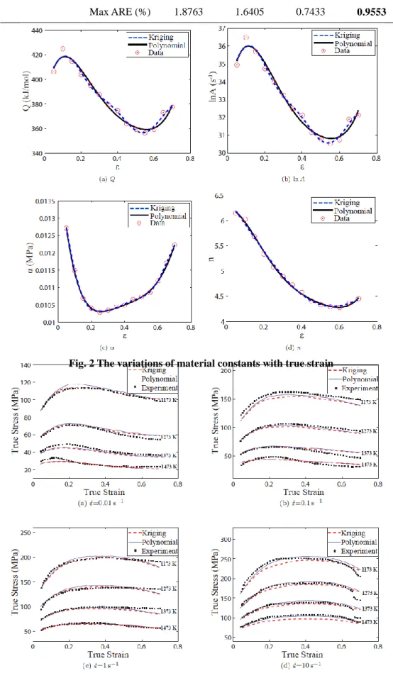
Figure 3 illustrates that flow stress predictions do not significantly differ by either of the two regression methods. The predicted flow stresses of 70Cr3Mo steel in Fig. 3 well follow the measured flow stresses. According to the usual validation approach in Ref. [5], r is

Table 4 Numerical validation of polynomial regression and regression Kriging models

Model Metric Q (kJ/mol) ln A(s^-1) α (MPa) n

Regression Kriging

R2

0.9875 0.9886 0.9995

0.4746 0.4846 0.1202

1.4956 1.3780 0.3170

regression

R2 ^{0.9746 0.9781 0.9972}

^0.9977

AARE (%) 0.7072 0.7199 0.2539

0.5310

Max ARE (%) 1.8763 1.6405 0.7433

0.9553

Fig. 2 The variations of material constants with true strain

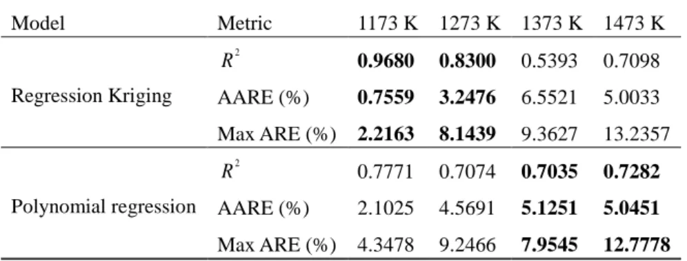
Fig. 3 Comparison of experimental and predicted flow stress at different strain rates Table 5 Validation results of surrogates at strain rate 0.01

Model Metric 1173 K 1273 K 1373 K 1473 K

Regression Kriging

R2

0.9680 0.8300 0.5393 0.7098

0.7559 3.2476 6.5521 5.0033

Polynomial regression

R2 0.7771 0.7074 0.7035 0.7282 AARE (%) 2.1025 4.5691 5.1251 5.0451 Max ARE (%) 4.3478 9.2466 7.9545 12.7778

Table 6 Validation results of surrogates at strain rate 0.1

Model Metric 1173 K 1273 K 1373 K 1473 K

Regression Kriging

R2 0.0362 0.5014 0.4634 0.6673 AARE (%) 5.2867 4.0067 6.3767 8.8093 Max ARE (%) 7.3012 5.1075 19.8601 16.5943

Polynomial regression

R2

0.5356 0.7986 0.2832 0.6493

3.5874 2.5276 8.0881 9.1843

Table 7 Validation results of surrogates at strain rate 1

Model Metric 1173 K 1273 K 1373 K 1473 K

Regression Kriging

R2

0.8543 0.8009 0.1055 0.8813

1.5538 2.1153 4.3735 1.6554

Polynomial regression

R2 0.8376 0.6830 0.4690 0.9156 AARE (%) 2.0477 3.0215 2.8236 1.4091 Max ARE (%) 6.2797 7.0077 11.4833 3.6286

Table 8 Validation results of surrogates at strain rate 10

Model Metric 1173 K 1273 K 1373 K 1473 K

Regression Kriging

R2 0.7645 0.8134 0.7096 -0.3309 AARE (%) 3.2959 2.8808 3.8241 8.6704 Max ARE (%) 6.9899 14.0143 22.8060 10.5659 Polynomial regression R²

0.8617 0.8143 0.6670 0.8554

AARE (%)

2.5867 2.5135 3.4838 2.7553

capability. On the contrary, the numerical validation results by the proposed validation scheme summarized in Tables 5 to 8 are relatively inferior. Note that neither polynomial regression nor regression Kriging is noticeably exceptional to the other. The individual validation results in Tables 5 to 8 imply that the constructed Arrhenius-type flow stress models in Ref. [5]

seemed fairly accurate overall, but they would actually result in large prediction errors when they are utilized at a certain temperature and strain rate condition.

5. Conclusion

To effectively incorporate strain into the Arrhenius- type constitutive equation, we leveraged regression Kriging as an alternative to other widely used regression technology, such as polynomial regression and artificial neural networks (ANNs). In addition, we employed validation procedures to thoroughly examine the goodness of prediction models not only for material constants but also flow stress. For illustration, we applied regression Kriging to the published data of 70Cr3Mo steel in Ref. [5]

and compared the prediction results of regression Kriging to those of polynomial regression.

For function approximation, regression Kriging relies on a basis that is determined by given data, whereas polynomial regression sticks to the predetermined monomial basis. As a result, regression Kriging tends to capture nonlinear behavior better than polynomial regression. For instance, regression Kriging demonstrated more accurate predictions than polynomial regression for relatively nonlinear material constants, such as Q and ln A. For flow stress model validation, we handled each set of flow stress data separately because one is typically concerned about flow stress prediction at a particular temperature and strain rate of interest. The proposed validation scheme showed that the ostensibly acceptable prediction analysis in Ref. [5] is actually misleading.

Although the regression models of the material

constants were trustworthy, the Arrhenius-type flow stress equations exhibited considerable prediction errors with both of the two regression techniques. Perhaps strain compensation alone is not sufficient for an Arrhenius-type constitutive model, and one may need to adjust the Zener- Hollomon parameter for better prediction.

Acknowledgement

This work was supported by a 2-Year Research Grant of Pusan National University.

REFERENCES

[1] Y. C. Lin, X. M. Chen, 2011, A Critical Review of Experimental Results and Constitutive Descriptions for Metals and Alloys in Hot Working, Mater. Des., Vol. 32, No. 4, pp. 1733~1759.

[2] H. Y. Li, D. D. Wei, Y. H. Li, and X. F. Wang, 2012, Application of Artificial Neural Network and Constitutive Equations to Describe the Hot Compressive Behavior of 28CrMnMoV Steel, Mater.

Des., Vol. 35, pp. 557~562.

[3] A. K. Gupta, S. K. Singh, S. Reddy, and G.

Hariharan, 2012, Prediction of Flow Stress in Dynamic Strain Aging regime of Austenitic Stainless Steel 316 Using Artificial Neural Network, Mater. Des., Vol. 35, pp. 589~595.

[4] A. K. Sulochana, C. Phaniraj, C. Ravishankar, A. K.

Bhaduri, and P. V. Sivaprasad, 2011, Prediction of High Temperature Flow Stress in 9Cre1Mo Ferritic Steel During Hot Compression, Int. J. Pres. Ves. Pip., Vol. 88, No. 11, pp. 501~506.

[5] F. Ren and J. Chen, 2013, Modeling Flow Stress of 70Cr3Mo Steel Used for Back-Up Roll During Hot Deformation Considering Strain Compensation, J.

Iron Steel Res. Int., Vol. 20, No. 11, pp. 118~124.

[6] M. L. Ma, X. G. Li, Y. J. Li, L. Q. He, K. Zhang, X.

W. Wang, and L. F. Chen, 2011, Establishment and Application of Flow Stress Models of Mg-Y-MM-Zr

Alloy, Trans. Nonferrous Met. Soc. China, Vol. 21, No. 4, pp. 857~862.

[7] M. R. Rokni, A. Zarei-Hanzaki, C. A. Widener, and P. Changizian, 2014, The Strain-Compensated Constitutive Equation for High Temperature Flow Behavior of an Al-Zn-Mg-Cu Alloy, J. Mater. Eng.

Perform., Vol. 23, No. 11, pp. 4002~4009.

[8] Y. K. Kim, J. O. Jo, J. P. Hong, and J. Hur, 2002, Application of Response Surface Methodology to Robust Design of BLDC Motor, KIEE EMECS, Vol.

12B, No. 2, pp. 47~51.

[9] A. I. Khuri and S. Mukhopadhyay, 2010, Response Surface Methodology, Wiley Interdiscip. Rev.

Comput. Stat., Vol. 2, No. 2, pp. 128~149.

[10] M. Murugesan, B. S. Kang and K. Lee, 2015, Multi- Objective Design Optimization of Composite Stiffened Panel Using Response Surface Methodology, Compos. Res., Vol. 28, No. 5, pp.

297~310.

[11] W. S. Cleveland and S. J. Devlin, 1988, Locally Weighted Regression: An Approach to Regression Analysis by Local Fitting, J. Am. Stat. Assoc, Vol.

83, No. 403, pp. 596~610.

[12] MathWorks, 2015, Curve Fitting Toolbox User's Guide

[13] I. Couckuyt, T. Dhaene, and P. Demeester, 2014, ooDACE Toolbox: A Flexible Object-Oriented Kriging Implementation, J. Mach. Learn. Res., Vol.

15, No. 1, pp. 3183~3186.

[14] I. Couckuyt, A. Forrester, D. Gorissen, F. D. Turck, and T. Dhaene, 2012, Blind Kriging: Implementation and Performance Analysis, Adv. Eng. Softw., Vol. 49, pp. 1~13.

[15] I. Couckuyt, F. Declercq, T. Dhaene, H. Rogier, and L. Knockaert, 2010, Surrogate-Based Infill Optimization Applied to Electromagnetic Problems, Int. J. Rf. Microw. C. E., Vol. 20, No. 5, pp. 492~501.