Tracer transport test in simple fractured media
ABSTRACT: Scientific visualization is an important method for understanding complex hydrologic processes. A series of experi- ments was conducted using two-dimensional fracture networks built of transparent plexiglass blocks as a new approach to process visualization. A digital monitoring method was used to visualize transport of a tracer in the fracture networks. The approach for visualizing tracer transport in fractured networks provided both quantitative and quantitative data. From the experiments con- ducted it was found that tracer spreading in fractured media was complex even in simple networks consisting of equally spaced finite fractures. The combined effects of fracture orientation and aperture variability resulted in the complex tracer spreading.
Key words: fracture, tracer, dispersion, visualization
1. INTRODUCTION
Solute transport in fractured rocks is a challenging area of study in subsurface hydrology because of the complexity of the processes involved. Previous studies noted situations with simple networks of fractured media where dispersion was complex (Schwartz and Smith, 1988). Certain network geometries provided principal directions of spreading at angles to the direction of mean flow and occasions where transverse spreading greatly exceeded longitudinal spread- ing. Kim et al. (2004) conducted a thorough numerical anal- ysis to understand this complex dispersion in the context of more variable networks and to evaluate the scaling between dispersion and characteristics of the network. Through sim- ulation trials, they examined how changes to the orientation of the overall network, fracture aperture, fracture connec- tivity, and fracture length influenced mass transport.
While numerical fracture models have been used to examine solute transport in a fractured media (Smith and Schwatrz, 1980; Schwartz et al., 1983), only a few laboratory studies have been performed with laboratory-scale fracture networks (Su et al., 2000, Lee et al., 2003). Many previous works have limitations in that they either used fractures having apertures much larger than real fracture apertures or plates to represent single fractures (Su et al., 2000).
The experiments presented in this paper are to study tracer transport in simple networks of closely spaced frac- tures. The main objectives were to monitor tracer transport
in fractured networks via visualization and to develop a methodology to robustly estimate tracer concentrations con- tained in small fractures. In general, fracture apertures of real fractured rocks are a few hundred microns wide, which made it difficult to conduct experiments for fractured rock systems. Furthermore, measuring contaminant concentra- tions in such small fractures is difficult. We constructed two-dimensional fracture networks using transparent plexi- glass blocks to create uniform fractures as a new approach to process visualization. Transport of a tracer was investi- gated through a series of experiments conducted using either a regular tracer solution or a tracer solution denser than water.
2. METHODS AND MATERIALS 2.1. Fracture Network
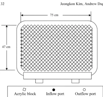
The fracture network built using uniform plexiglass blocks of 2.54-cm long, 2.54-cm wide, and 1.27-cm deep (Eastech Plastics, Worthington, Ohio) had 2 sets of fractures oriented at positive and negative 45 degrees with respect to the hor- izontal plane. Figure 1 shows the schematic of the 45-degree network. The average fracture aperture for the 45-degree network was 200 microns. The 45-degree network had 11 inflow and 11 outflow ports for injecting and removing flu- ids, respectively.
The magnitude of fracture apertures determines the per- meability of the fractures. If fractures are idealized as par- allel plates, each having a constant aperture, then, the hydraulic conductivity, Kf, of a parallel-plate fracture of aperture, 2b, is given for smooth laminar flow conditions (Re < 2300) by the following equation (Gale, 1982):
(1) where ρ is the fluid density, g is the gravitational constant, and µ is the dynamic viscosity. Then, flux can be calculated by the Darcy’s law.
2.2. Experimental Methods
Kroger red food coloring (Kroger Company, Cincinnati,
Kf ρg
12µ --- 2( )b 2
= Jeongkon Kim
Andrew Duguid Franklin W. Schwartz
Korea Institute of Water & Environment, Korea Water Resources Corporation, Daejeon 305-730, Korea Department of Civil and Environmental Engineering, Princeton University, Princeton, New Jersey, U.S.A.
Department of Geological Sciences, The Ohio State University, Columbus, Ohio, U.S.A
*Corresponding author: [email protected]
Ohio), which doesn’t affect density and viscosity of the solution, was used for the tracer solution used in this study.
Among many trials we conducted, 2 experiments to be pre- sented are summarized in Table 1. Two kinds of experiments were run using the fracture networks: flooding and plume experiments. The flooding experiments were conducted by
injecting tracer into all of the inflow ports in the model, while the plume experiments by injecting tracer into the network from one or a few of the inflow ports and injecting water into all other inflow ports.
Because of the small aperture sizes, the volume of the network was small. With this small network volume, the pulsing of the peristaltic pump caused serious pressure tran- sients. In order to eliminate the effects of the pump, a con- stant-head reservoir was constructed. The reservoir received flow from the pump and delivered it to the injection man- ifold. To eliminate the pressure transients created by the pump, the reservoir was open to the atmosphere. Water was pumped into the reservoir and allowed to spill over the sides. This ensured that the head in the reservoir remained constant at all times. The overflow was collected and returned to the reservoir that fed the pump. Two constant-head res- ervoirs were built. One was used to control the inflow of water to the network. The other was used to inject tracer into the network. The outflow head was controlled by means of a small open reservoir that could be raised or low- ered to achieve the desired pressure gradient across the frac- ture network. Figure 2 shows the experimental setup for the injection of water and tracer into the network.
A digital monitoring approach, similar to that employed by Schincariol et al. (1993) and Seol et al. (2001), was devel- oped. One most important advantage that this method pro- vided was that the flow regime in the network was not perturbed during the experiments. This feature was critical to the success of the experiments considering the small vol- ume of water flowing through fractures in the network. As the tracer moved across the fracture network during the experiments, images of the plumes in the experiments were collected using a Nikon 990 CCD digital camera. The cam-
Fig. 1. A schematic of the fracture network.
Table 1. Summary of experimental data.
Experimental
type Influent head
(cm) Effluent head
(cm) Head difference
Flooding 164.0 74.5 (cm)89.5
Plume 164.0 77.0 87.0
Fig. 2. Schematic of the experimental injection setup showing reservoirs, pump, constant-head reservoirs, mani- folds, network, and direction of fluid flow.
era was connected to a Digisnap 1000 remote shutter release (Harbortronics, Gig Harbor, Washington), which was pro- grammed to make the camera take a series of pictures over time. The use of the remote shutter release eliminated the small variations in photos that could be created with manual operation.
The fracture aperture in the network was a few hundred microns wide, which made it almost impossible to photo- graph the tracer in the network. To overcome this difficulty, instead of taking shots at fractures at zero angles, the pho- tographs were taken at an angle of about 20 degrees with respect to the face of the network. Then, fractures appeared to be a few thousand microns wide. This method of imag- ing fractures from an angle made it possible to observe the tracer passing through the tiny fracture apertures.
3. RESULTS AND DISCUSSION 3.1. Flooding Experiment
The flooding experiments were to collect background information on the characteristics of the networks, which provided a basis for interpreting the plume experiments.
Furthermore, the quantitative analysis for tracer concentra- tions were explored using the light transmittance values for specified fractures measured at maximum tracer concentra- tions.
Figure 3 shows tracer distribution for the flooding exper- iment. The networks were marked with small colored stick- ers to identify the locations of fractures that were used for data collection as shown in Figure 3. Six sets, each con- sisting of 6 vertical points, in the horizontal direction are located (from left to right) at 7, 17, 28, 39, 50, and 60 cm from the inflow boundary of the network. The 6 vertical points are located at 7.2, 14.4, 21.6, 28.7, 35.9 and 43.1 cm measured from the top boundary (Fig. 3). The points were also arranged in a vertical line on the network.
The tracer distribution shown in Figure 3 was assumed to be steady-state conditions. Then, the steady-state tracer concentration in the fractures must be uniform. However, the intense of tracer color were not uniformly distributed as shown in Figure 3. The variation in the tracer color intensity was caused by different angles between the camera and the fractures. For example, fractures located in left and right sides of the network show relatively darker red color than those located elsewhere due to dif- fering angles.
Due to the symmetry of the fracture network for the 45- degree network, the quality of visualization was similar for the two fracture sets. There were some low permeable frac- tures as evidenced by the fractures showing no tracer, which implies that the networks were heterogeneous. The hetero- geneity observed in the two networks was due to variability in fracture aperture. Although many efforts and cautions
were exercised to make homogeneous fracture networks (i.e., equal aperture), apparently aperture heterogeneity was created to some degree during the construction. Two major causes, among many factors that contributed to the creation of the aperture variability, are unequal block sizes due to manufacturing tolerance and the liquid resin used to fix the blocks in the network. Visual observations made before and after the experiments revealed that a number of factures were, in fact, either fully or partially clogged, confirming that the later should be responsible for the fractures with no tracer.
3.2. Plume Experiment
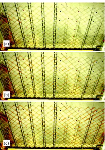
The plume experiment provided information on tracer plume development in the fracture networks. Figure 4 shows tracer distribution for the plume experiment, con- ducted by allowing the tracer to flow into the network through an injection port located in the upper left side of the network. The plume reached the red reference points (4 blocks away from the boundary) horizontally with no significant lateral spreading (Fig. 4a). This initial plume was created through a fast flow path in the direction of flow. After 120 minutes, it had spread laterally across the tank and spread vertically across the entire thickness of the network within a distance of eight blocks (29 cm) from the influent port (Fig. 4b). Note, however, that the low permeability zones discussed in flooding experiment were bypassed (Fig. 4b) and were gradually influenced by the tracer as the experiment progressed (Fig. 4c). Overall, the tracer concentrations were lower than those obtained for the flooding experiment as evidenced by lower intensity of the plumes (compare Figs. 3 and 4c).
Dispersion is a process that causes a zone of mixing between two fluids with differing solute concentrations (Domenico and Schwartz, 1998). The effect of dispersion is to spread mass outside of the space that the mass would occupy due to flow alone. Spreading in the direction of flow is known as longitudinal dispersion, and spreading normal to the direction of flow as transverse dispersion.
In problems of groundwater contamination, dispersion is important because it can substantially reduce an initial groundwater contaminant concentration through dilution.
Many laboratory and field studies have shown that for porous media, longitudinal dispersion leads to much more significant mixing than transverse dispersion (Domenico and Schwartz, 1998). As a general rule then, transverse dispersion has been considered to be an ineffective mix- ing process. This idea has been extended to fractured rocks. Investigators looking at contaminant transport in fractured rocks generally disregard vertical transverse dispersion as an attenuation mechanism (Mckenna et al., 2003).
Previous studies, however, noted situations with simple
networks of fractured media where transverse dispersion was significant. For example, Kim et al. (2004) through numerical experiments found that grid effect resulting from a direct consequence of orientations of the fracture network created enhanced vertical spreading in fractured media.
They also found that as fracture spacing increased, trans- verse dispersion increased as well. The results of the plume experiment also showed significant transverse dispersion, with the plumes spreading across the entire depth of the net- work (Fig. 4).
3.3. Toward Quantitative Analyses
As the tracer moved across the fracture network during the experiments, images of the plumes in the experiments were collected. The visual observation provided qualitative information on tracer spreading in the fracture networks. As mentioned earlier, one of the most important advantages that this method provided was that the flow regime in the network was not affected. However, it is usually necessary to obtain quantitative information such as tracer concentra- tion in fractures, which was not an easy task. A few different approaches for quantitative data collection were examined.
The most common method is collecting water samples to measure tracer concentrations using a spectrophotometer.
This method, however, was not appropriate because the sample volume required for the analysis was too large com- pared to the total water volume in the network. For exam- ple, collecting a volume of 0.5 ml per sample at several locations caused significant hydraulic head drop. This reduc- tion in head would have meant that the flow regime in the network would not have been consistent throughout the experiments.
As an alternative, a digital monitoring approach similar to Schincariol et al. (1993) was developed. The images taken during the experiments were analyzed using Adobe Photo- shop software. The histogram tool in Photoshop measures colored light transmittance in an image or a selected portion of an image. The method required choosing an area on a fracture in an image and zooming in on it. The area was selected using the marquee tool and copied to another file.
By using the histogram tool on the new file, colored light data could be measured and recorded. A master picture of each point was created, and this image was used as a map to make sure that the same points on each photo were used.
This approach ensured that changes in transmittance were due to movement of tracer in the networks, not movement of the sample point on the image. The master image was also used as a map to place the marquee tool in the correct location.
Tracer concentrations were calculated using green light transmittance values taken from the digital images of the plumes (Seol et al., 2001). The light transmittance at or before the start of an experiment was correlated to 0% tracer con- centration. The transmittance data from the flooding exper- iments were assumed to be 100% concentrations, Cmax. Then, normalized tracer concentrations, C/Cmax, for each fractures were calculated by dividing the transmittance from a plume experiment by the transmittance data from a flooding exper- iment. The method converted transmittance data into normal- ized concentrations expressed as a fraction of the maximum concentration. One, however, must be careful as the steady- state tracer intensity was not uniform due to differing angles between the camera and fractures in the network (Fig. 3).
That is, the transmittance data from the flooding experi-
Fig. 4. Tracer distributions for plume experiment at (a) 60, (b) 120, and (c) 420 minutes.
Fig. 3. Tracer distributions from flooding experiment at 4140 minutes.
ments assumed to be 100% concentration is location spe- cific. Therefore, the normalized tracer concentration, C/Cmax, for each fractures must be calculated by using the transmit- tance data from a plume experiment and the transmittance data from a flooding experiment at each corresponding point in the network.
The change in transmittance of the tracer concentration was not linear with respect to change in concentration.
Because the method for changing the transmittance into concentration assumed that the change was linear, the con- centration value had to be corrected. The correction that was used was the equation of the line of the actual versus the calculated concentrations. The control experiment con- sisted of a set of vials with known concentrations of tracer.
The vials were photographed and the concentration was cal- culated using the light transmittance method. The scale used in this study ran between 0 (0 percent) concentration representing the transmittance before any tracer entered the network and the 1.0 (100 percent) concentration represent- ing the transmittance of the completely flooded network.
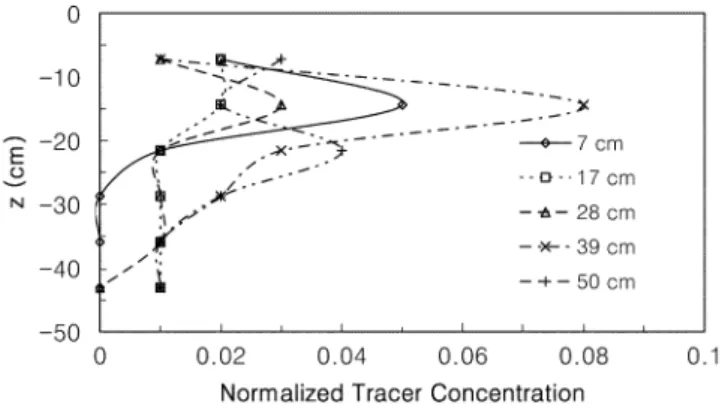
Collecting concentration data was time consuming con- sidering that tracer concentration at each point should be calculated using individual Cmax value. Figure 5 shows a breakthrough curve obtained from the transmittance data for a fracture located at the outflow port in flooding exper- iment. Figure 6 presents tracer concentrations estimated for the fractures located right above the colored stickers for plume experiment at 420 minutes after start of experiment.
Each line represents tracer concentrations estimated along the vertical direction at a given horizontal location. Note that the tracer concentrations are not necessarily continuous due to aperture heterogeneity as discussed earlier. Individ- ual data points were connected only for illustration pur- poses. Although there are exceptions, tracer concentrations, in general, were higher for the fractures located close to the source (-15 cm). It is obvious that tracer at deeper locations was detected for the data sets located far away from the source due to vertical spreading.
4. CONCLUSIONS
Fracture apertures of real fractured rocks are a few hun- dred microns wide. Thus, measuring contaminant concen- trations in such small fractures is difficult. We constructed two-dimensional fracture networks using transparent plexi- glass blocks as a new approach to process visualization.
Transport of a tracer in the fracture networks was monitored using a digital visualization method. Scientific visualization is an important method for understanding complex hydro- logic processes. The approach developed for visualizing tracer transport in fractured networks provided both quali- tative and quantitative data. It was observed that tracer spread- ing in fractured media was complex even in simple networks consisting of equally spaced finite fractures, resulting from the effects of grid orientation and aperture variability.
REFERENCES
Domenico, P.A. and Schwartz, F.W., 1998, Physical and Chemical Hydrogeology. John Wiley and Sons, Inc., New York, 455 p.
Gale, J., 1982, Assessing the permeability characteristics of fractured rocks. Special Publication, Geological Society of America, 189, 163−181.
Kim, J., Schwartz, F.W., Smile, L. and Ibaraki, M., 2004, Complex dispersion in simple fractured media. Water Resources Research, 40, 1029−1039.
Lee, J., J.M. Kang, and J. Choe, 2003, Experimental analysis on the effects of variable apertures on tracer transport, Water Resources Research, 39(1), 1015, doi:10.1029/2001WR001246.
McKenna, S.A, Walker, D.D. and Arnold, B., 2003, Modeling dis- persion in three-dimensional heterogeneous fractured media at Yucca Mountain. Journal of Contaminant Hydrology, 62−63, 577
−594.
Schincariol, R.A., Henderic, E. and Schwartz, F.W., 1993, On the application of image analysis to determine concentration distri- butions in laboratory experiments. Journal of Contaminant Hydrol- ogy, 12, 3, 197−215.
Seol, Y., Schwartz, F.W. and Lee, S., 2001, Oxidation of bnary DNAPL mixtures using potassium permanganate with a phase transfer catalyst. Ground Water Monitoring and Remediation, Spring, 124− Schwartz, F.W. and Smith, L., 1988, A continuum approach for mod-132.
eling mass transport in fractured media. Water Resources Research, 24, 8, 1360−1372.
Schwartz, F.W., Smith, L. and Crowe, A.S., 1983, A stochastic anal-
Fig. 5. Normalized blue light data obtained for a fracture from flooding experiment.
Fig. 6. Normalized tracer concentrations estimated for selected fractures from plume experiment at 420 minutes.
ysis of macroscopic dispersion in fractured media. Water Resources Research, 19, 5, 1253−1265.
Smith, L. and Schwartz, F.W., 1980, Mass Transport. 1. An analysis of the influence of fracture geometry on mass transport in frac- tured media. Water Resources Research, 20, 9, 303−313.
Su, G.W., Geller, J.T., Pruess, K. and Hunt, J., 2000, Overview of
preferential flow in unsaturated fractures. Dynamics of Fluids in Fractured Rock, Geophysical Monograph, 122, The American Geophysical Union, Washington, D.C.
Manuscript received May 6, 2005 Manuscript accepted June 14, 2006