Elasticity Signal and Image Processing Sensor and Algorithms for Tissue Characterization

(1)

SSSeeennnsssooorrrsss &&& TTTrrraaannnsssddduuuccceeerrrss s

http://www.sensorsportal.com

Elasticity Signal and Image Processing Sensor and Algorithms for Tissue Characterization

1 Jong-Ha LEE, ¹Hee-Jun PARK, ²Nyeon-Sik EUM, ³Hyuk-Jun Yoon and ³Yoon-Nyun KIM

1 Department of Biomedical Engineering, Keimyung University, School of Medicine, Daegu, South Korea

2 303 Bl Center, Kyungpook National University U-BioMed Inc., Daegu, South Korea

3 Department of Cardiology, Department of Internal Medicine Keimyung University Dongsan Medical Center, Daegu, South Korea

1 Tel.: (82)-53-580-3836, fax: (82)-53-580-3846

1 E-mail: [email protected]

Received: 29 January 2014 /Accepted: 30 January 2014 /Published: 31 January 2014

Abstract: The tissue inclusion parameter estimation method is proposed to measure the stiffness as well as geometric parameters. The estimation is performed based on the elasticity image obtained at the surface of the tissue using an optical based elasticity imaging sensor. A forward algorithm is designed to comprehensively predict the elasticity image based on the mechanical properties of tissue inclusion using finite element modeling.

This forward information is used to develop an inversion algorithm that will be used to extract the size, depth, and Young's modulus of a tissue inclusion from the elasticity image. We utilize the artificial neural network (ANN) for inversion algorithm. The proposed estimation method was validated by the realistic tissue phantom with stiff inclusions. The experimental results showed that the proposed estimation method can measure the size, depth, and Young's modulus of a tissue inclusion with 0.58 %, 1.12 %, and 0.51 % relative errors, respectively. A small-scale of breast cancer patient experiments is also presented. The obtained results prove that the proposed method has potential to become a screening and diagnostic method for breast tumor.

Keywords: Tumor detection, Artificial palpation, Lesion characterization, Elasticity sensor, Biomimetic sensor, Young’s modulus.

1. Introduction

Breast nodule stiffness or elasticity is an acknowledged indicator of breast health, with increased tissue stiffness pointing to an increased risk of breast cancer. During the past two decade, various methods have been devised for measuring or estimating the soft tissue elasticity [1]. Generally it is

called elasticity imaging. Elasticity imaging is currently performed using magnetic resonance elastography (MRE), atomic force microscopy (AFM), and ultrasound imaging. MRE is a dynamic approach where external oscillation is applied to the material and acoustic strain waves caused by the oscillation are visualized [2]. AFM has also been utilized to detect tissue elasticity; however, this is for

(2)

small local area measurement [3]. Both MRE and AFM are extremely expensive and cumbersome. The ultrasound is perhaps the most intensely investigated area for elasticity imaging [4, 5]. The ultrasound can be divided into three cases: elastography, transient elastography, and sonoelastography. In elastography, compression is applied to the tissue then pre- compression and post-compression echo return signals are compared using correlation techniques to calculate the strain map in the tissue [6, 7]. Transient elastography uses a low frequency transient vibration to create displacements in tissue, which are then detected using pulse-echo ultrasound.

Sonoelastography uses real-time ultrasound Doppler techniques to image the vibration pattern resulting from the propagation of low frequency shear wave that are propagated through the [8]. The research with elasticity imaging shows that elastic modulus information has the potential of distinguishing malignant and benign tumors [9, 10]. It is difficult to compare each technology because both technologies are at their infancy, however, from the physics point of view, the ultrasound will suffer from limited contrast and resolution problems [11].

Palpation of the breast to determine breast stiffness is an established screening method for assessing breast health. Women are advised to undergo a clinical breast examination (CBE) [12]. At present, physicians write up their findings, which are accompanied by a hand drawing of the breast mass.

Thus, it is difficult to quantify the tactile sensation presented by the breast tumor. The efficacy of CBE is also limited by the experience of the physician. A noninvasive method for recording and estimating the stiffness would offer great clinical utility. The stiffness can be quantified using Young’s modulus.

In addition to increased tissue stiffness, geometric parameters such as size and depth of the stiff region are important factors in assessing the tumor. The combined knowledge of tumor stiffness and geometry would aid tumor identification and help physicians select an appropriate treatment strategy.

The objective of this research is to develop a methodology to estimate the mechanical properties of an embedded tumor based on the data obtained by the elasticity imaging sensor (EIS). We proposed the design concept for the EIS and elasticity image processing methodology used to quantify various parameters—size, depth, and Young's modulus—of an embedded tumor with a geometry representative of breast pathology. For this purpose, finite element method (FEM) and neural network (NN) algorithm are utilized. FEM is used to generate simulated elasticity image on the tissue surface over different embedded tumor parameters in the idealized breast model. We employ NN algorithm to map the simulated elasticity image to the tumor parameters.

We then compare NN training results with those obtained from a realistic tissue phantom. The proposed characterization method was validated by the realistic tissue phantom with inclusions to emulate the tumors and real clinical trials.

2. Sensor Design and Sensing Principle 2.1. Elasticity Imaging Sensor

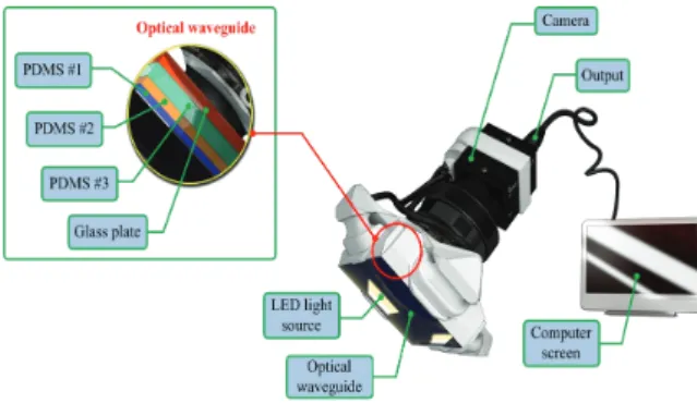
The EIS incorporates an optical waveguide unit, a light source unit, a high resolution camera unit, and a computer unit. The optical waveguide is the system’s main sensing probe. The waveguide is composed of polydimethylsiloxane (PDMS), which is a high- performance silicone elastomer. In the current design, the waveguide needs to be flexible and transparent, and PDMS meets this requirement. To reach the level of sensation of human touch, we emulated the tissue structure of the human finger. The human finger tissue is composed of three layers with different elastic moduli, specifically the epidermis, dermis, and subcutaneous layer. The epidermis is the hardest layer, with the smallest elastic modulus, and it is approximately 1 mm thick. The dermis is a softer layer, and it is approximately 1 to 3 mm thick. The subcutaneous is the softest layer and fills the space between the dermis and bone. It is mainly composed of fat and functions as a cushion when a load is applied to the surface. Due to the difference in hardness of each layer, the inner layer deforms more than the outmost layer when the finger presses into an object. To emulate this structure, three PDMS layers with different elastic moduli were stacked together.

PDMS layer 1 is the hardest layer, the PDMS layer 2 is the layer with medium hardness, and the PDMS layer 3 is the layer with the least hardness. The height of each layer is approximately 2 mm for PDMS layer 1, 3 mm for PDMS layer 2, and 5 mm for PDMS layer 3. Fig. 1 shows the schematic of the proposed sensor.

Fig. 1. The schematic of the elasticity imaging sensor (EIS).

The high resolution camera was a mono-cooled complementary camera with an individual pixel size of 4.65 μm (H) × 4.65 μm (V). The maximum lens resolution was 1,392 (H) × 1,042 (V) with an angle of view of 60°. The camera was placed below an optical waveguide. A heat-resistant borosilicate glass plate was placed between the camera and the waveguide to sustain an optical waveguide without losing the camera resolution. The internal light source was a micro-LED with a diameter of 3 mm.

There were four LED light sources placed on four

(3)

sides of the waveguide to provide sufficient illumination. The direction and incident angle of light were calibrated to be totally reflected in the waveguide.

2.2. Elasticity Imaging Principle

The proposed EIS operates on the principle of total internal reflection (TIR). According to Snell's law, if two mediums have different refractive indices, and the light is shone through those two mediums, then a fraction of light is transmitted and the rest is reflected. If the incident angle is above the critical angle, then TIR occurs. In the current system design, since the waveguide is surrounded by the air, and has a lower refractive index than PDMS layers, the incident light directed into the waveguide is totally reflected in the waveguide. The waveguide is transparent and flexible. Consequently, if a waveguide is compressed by an external force towards a stiff inclusion, the contact area of the waveguide deforms and causes the light to scatter.

The scattered light is then captured by the high- resolution camera and saved as an image. Thus, the basic principle of tactile sensation imaging lies in capturing of the light scattered due to the inclusion.

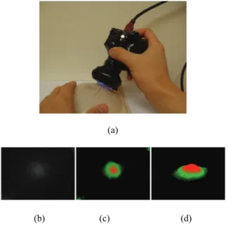
Fig. 2 shows the EIS and obtained elasticity image.

(a)

(b) (c) (d) Fig. 2. (a) EIS and breast phantom. (b) Obtaining elasticity image of a tissue inclusion (Raw gray-scale elasticity image), (c) Color visualization, (d) 3-D reconstruction.

3. Tissue Inclusion Characterization Algorithm

The idealized model used to estimate the various tumor parameters derived from the elasticity image is shown in Fig. 3. The assumptions used in the proposed idealized model are as follows.

1) Most breast tumors are found in the upper outer quadrant of the breast where the tissue is relatively thin and flat [13]. Therefore, in our model, the tissue is approximated as a slab of material of constant thickness that is fixed to a flat, incompressible chest wall.

2) The inclusion is assumed to be spherical and stiffer than the surrounding tissue. Wellman et al.

used a breast modeling algorithm to investigate this assumption [14]. In clinical tests, they found that the results matched well with their breast modeling results under this assumption.

3) We assume that both the tissue and the inclusion are linear and isotropic. Glandular and adipose tissues, which account for most of the breast tissue, are well modeled by isotropic materials [15].

4) In this model, the indentation is made by the sensing probe of the EIS with finite length. The interaction between the sensing probe and the tissue is assumed to be frictionless.

In the next section, we devise a methodology for estimating three parameters of the embedded inclusion: size (d), depth (h) and Young’s modulus (E). The estimation of these parameters will be extracted from the EIS elasticity image obtained at the tissue surface.

Fig. 3. The tumor diameter (d), the depth (h), and the Young’s modulus (E).

3.1. Forward Modeling

We use finite element method (FEM) to investigate the elasticity image obtained by the EIS on the surface of the tissue with embedded inclusion.

Fig. 4 presents a graphical representation of the FEM model. The FEM model consists of tissue, inclusion, and sensing probe of EIS. The FEM model comprises 3000 finite elements. The FEM is performed by the following assumptions [16].

1) The biological tissue and inclusion are elastic and isotropic. It means the properties of a material are identical in all directions.

2) The Poisson’s ratio of each material is set to 0.49 because the breast can be considered an incompressible material. The incompressible material means the material incapable of or resistant to compression.

(4)

3) The biological tissue is assumed to be sitting on non-deformable hard surfaces like bones.

4) The tissue cross-section is a square with dimensions 120 mm120 mm. The sensing probe of the EIS is a square shape with dimensions of 25 mm25 mm, which corresponds to the sensing probe size in the laboratory design.

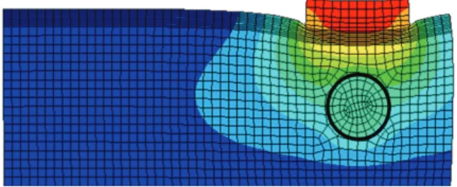
All are modeled using SOLID95 3D elements available in ANSYS. Appropriate surface-to-surface contact elements have been defined in the ANSYS database model. The cross-section FEM meshed model with tissue, inclusion, and sensing probe of the EIS is shown in Fig. 3.

Fig. 4. FEM model of an 8 mm diameter inclusion embedded in tissue 20 mm thick. The inclusion is located 5 mm beneath the tissue surface. The sensing probe of the EIS is also shown in top of the tissue model.

3.2. Elasticity Image from FEM

If the sensing probe compresses against the tissue containing a stiff inclusion, the deformation occurs.

In the FEM, we capture the deformed shape in response to different parameters of inclusions. To quantify the FEM elasticity image, we use the following three definitions: maximum deformationO¹_FEM , total deformationO_FEM² , and deformation area O_FEM³ of sensing probe. The maximum deformation O¹_FEM is defined as the maximum displacement of elements from the bottom surface of the sensing probe. The unit of the maximum deformation is mm. The total deformation

2

OFEM is defined as the displacement summation of elements from the bottom surface of the sensing probe. The unit of the total deformation is mm. The deformation area O³_FEM is defined as the deformed bottom surface area of the sensing probe where the displacement of finite elements is greater than 0. The unit of the deformation area is mm².

To investigate the relationship between (d,h,E) and (O¹_FEM,O_FEM² ,O_FEM³ ), 512 input data sets are randomly generated as inputs of FEM. Among 134 input data sets, 9 input data sets are used to build the calibration tissue phantom. 512 output data sets corresponding to 512 input data sets are being generated through FEM. To visualize 134 data sets in 3D space, output data sets are rescaled to [0:255] and

displayed as colored circles at the locations specified by three inputs (d,h,E). The area of each marker is determined by the values in the vector and the colors of each marker are based on the values from 0 to 255. From the results, we notice that as the size of inclusion increases, the elasticity image increases as the effect of bigger inclusion will cause more change in the sensing probe deformation. As the depth of inclusion increases, the elasticity image decreases as the effect of stiff inclusion gets reduced and sensing probe presses the soft tissue. As the Young's modulus of inclusion increases, the elasticity image increases as the stiff inclusion makes the sensing probe to deform more.

3.3. Calibration Mapping

Since the FEM measures the quantity of the sensing probe deformation and the EIS measures the quantity of the dispersed light due to the sensing probe deformation, it is necessary to relate the FEM elasticity image and EIS elasticity image. This is the calibration process. For this purpose, we obtained elasticity image of calibration phantom using both FEM and EIS. The calibration phantoms consist of three phantoms, size, depth, and hardness phantoms.

Each phantom contains three inclusions, resulting in a total of nine inclusions. Every inclusion has three parameters (d ,h,E ). The Young’s modulus of background tissue phantom is 5 kPa, and the height is set at 20 mm.

To map the elasticity image of EIS to elasticity image of FEM, first, we simulated elasticity image of nine inclusions using FEM. The elasticity image was then quantified by (O¹_FEM, O_FEM² , O_FEM³ ). From the results, we clearly see that if d and E are increasing, O¹_FEM and O_FEM³ are increasing.

However, we can observe that if h is increasing,

2

OFEM is decreasing. The elasticity image on the inclusions in the calibration phantoms was also obtained by the EIS. The EIS elasticity image is quantified by (O_TSIS¹ , O_TSIS² , O_TSIS³ ). It can be observed that the results show the similar pattern with the FEM case. To investigate the relationship between FEM elasticity image and EIS elasticity image, we generated graphs of ( O¹_FEM ; O_TSIS¹ ), ( O_FEM² ; O_TSIS² ), and ( O_FEM³ ; O_TSIS³ ). Linear regression was used to model the relationship between FEM elasticity image and EIS elasticity image.

3.4. Inversion Algorithm

The goal of the elasticity image processing is to estimate inclusion's size, depth, and Young's modulus using the elasticity image. In the forward modeling,

(5)

we generated 512 input data sets (d , h, E) and investigated its output data sets ( O¹_FEM , O_FEM² , O_FEM³ ). Now, we design the inversion algorithm to estimate (d , h, E) using (O¹_FEM,O_FEM² ,O_FEM³ ). To achieve this purpose, first we need an inversion algorithm training using 512 data sets generated in the forward modeling. In this paper, one of the statistical learning algorithms, neural network (NN), is utilized for the inversion algorithm.

In this study, we have taken multilayered neural network. Multilayered neural network consists of neurons united in layers. Each i layer is connected with i-1 and i+1 layers and neurons in layer are not connected to each other. In the structure, too many neurons would lead to over-fitting and great variance of mean squared error (MSE) results, but not enough neurons would cause high MSE results. Thus numbers of neurons and layers were set experimental way to 3 layers as follows: 1) 1^st layer: 25 neurons, sigmoid activation function, 2) 2^nd layer: 10 neurons, sigmoid activation function, 3) 3^rd layer: 7 neurons, linear activation function. For training the NN, two different algorithms were considered. The first one is the Levenberg-Marquardt algorithm (LMA) and the second one is the Scaled Conjugate Gradient algorithm (SCGA). The LMA is a very popular curve-fitting algorithm used in many software applications for solving generic curve-fitting problems. The LMA interpolates between the Gauss–

Newton algorithm (GNA) and the method of gradient descent. The LMA is more robust than the GNA, which means that in many cases it finds a solution even if it starts very far off the final minimum. On the other hand, for well-behaved functions and reasonable starting parameters, the LMA tends to be a bit slower than the GNA. LMA can also be viewed as Gauss–Newton using a trust region approach.

Below is the summary of the LMA.

5. Experimental Results

For the validation of the network model, we used two types of cross validation method.

5.1. Validation Method

The first one is the hold out validation (HOV) and the second one is the leave one out cross validation (LOOCV). Hold-out validation (HOV) is the most common validation method of the NN. In this method, an independent test set is preferred to avoid over-fitting. A natural approach is to split the available data into two non-overlapped parts: one for training and the other for testing. The test data is held out and not looked at during training. HOV avoids the overlap between training data and test data, yielding a more accurate estimate for the

generalization performance of the algorithm. The downside is that this procedure does not use all the available data and the results are highly dependent on the choice for the training/test data split. In the current 512 data sets, we use 9 data of calibration phantom as test data. Leave-one-out cross-validation (LOOCV) is a special case of k-fold cross-validation where k equals the number of instances in the data. In other words, in each iteration, nearly all the data except for a single observation are used for training and the network model is tested on the single observation. An accuracy estimate obtained using LOOCV is known to be almost unbiased but it has high variance, leading to unreliable estimates. It is still widely used when the available data are very rare, especially in bioinformatics where only dozens of data samples are available.

The final estimation error is average of iterations’

estimation error. In this study, the mean squared error (MSE) is used to represent the estimation error. The MSE is computed as follows. Let P be input data matrix, T be output data matrix and Y be network’s output data matrix. Then MSE e_j is calculated as below.

2 1

1 ⁿ ( ) 100 (%)

j ij ij

i

e T Y

n 

    ⁽¹⁾

where is the test data number and is the output number.

5.2. Test Results

In this section, two training algorithms, LMA and SCGA, are validated using two validation methods, HOV and LOOCV. The result shows that LMA works with higher accuracy than SCG. Also there is no need to train network more than 100 iterations.

The test results of the NN are averaged with 10, 50, and 100 experiments. Also from the results, we notice that both SCGA and LMA’s train results are good; however, LMA seems to be over-fitted already after 100 iterations because of high errors. Best result shows SCG with LOOCV at 100 iterations. The results are 0.58 % MSE of size, 1.12 % MSE of depth, and 0.51 % MSE of Young's modulus.

5.3. Sensitivity and Specificity Tests

In this section, the sensitivity and specificity of the EIS are investigated. To measure the sensitivity and specificity of the EIS, we used the tissue phantom which contains eight tissue inclusions (MammaCare Corp., FL). The sensitivity of the EIS was obtained by calculating true-positive results, Tp, and false- positive results, Fp, through detecting eight tissue inclusions in the phantom using the EIS. To measure

(6)

the specificity of the EIS, the number of true negative results, Tn, and number of false-negative results, Fn, was calculated while scanning the tissue phantom without tissue inclusions. The experimental results show that the number of true-positive results, Tp, was six and the number of false-negative results, Fn, was two, resulting in a sensitivity of 75 % for the EIS. For the specificity, the number of true-negative results, Tn, was seven and the number of false-positive results, Fp, was one. Thus, the specificity is 87.5 %.

These are the preliminary results of the EIS sensitivity and specificity test. If we increase the number of samples, then we may collect more precise EIS sensitivity and specificity data. The relationship between sensitivity and specificity can be illustrated by the receiver operating characteristic (ROC) curve, which is a graphical plot of the true-positive rate (sensitivity), against the false-positive rate (1-specificity). A ROC curve facilitates advanced analysis of the classification accuracy of a diagnostic method.

Generally, the closer the ROC curve follows the left-hand border of the graph and then the top border of the graph, the more accurate the test. The closer the curve comes to the 45 degree diagonal of the graph, the less accurate the test. The shape of the ROC curve can be determined by the area under the curve (AUC). Thus, the AUC can be used as a measure of test accuracy. A 100 AUC of 1 represents a perfect test and an AUC of 0.5 represents a worthless test. An experimental result that gives a larger AUC indicates a better method than one with a smaller area. In general terms, an AUC above 0.8 is considered excellent, between 0.75 and 0.8 is very good, between 0.7 to 0.75 is good, between 0.6 to 0.7 is poor, and between 0.5 to 0.6 is a fail (Roques et al., 2000). Because the AUC of the EIS ROC curve is 0.835, the EIS experimental results can be considered as good.

5.4. Clinical Trials

Clinical studies of the EIS are currently being conducted at the Temple University Hospital. Here, we present just a few pilot results. Three patients presented with a lesion that was initially detected by another modality (mammography, ultrasound, or manual palpation). When performing the EIS scans, the doctor already knew where the lesions were located. For each lesion, 30 elasticity images were obtained and the estimated parameters were averaged. The size truth values were provided by mammogram, and malignancy results were obtained from the pathology reports. The size of the lesion of the patient 1 was 3.28 mm and the estimated value using the proposed method was 3.34 mm. The relative estimation error is 1.79 %. In the case of the patient 2, the size of the lesion was 5.34 mm and the estimated value was 5.44 mm. The relative estimation error is 1.83 %. For patient 3 case, the size of the lesion was 4.12 mm and the estimated value was

4.22 mm, resulting in the 2.36 % relative estimation error. Regarding the hardness estimation of the lesions, malignant breast lesion of the patient 1 had increased Young’s modulus (135 kPa), compared to benign lesions (62 kPa and 78 kPa, patient 2 and 3).

The elasticity information was correlated with the malignancy data from the pathology reports.

6. Conclusions

In this paper, an optical based tissue inclusion parameter estimation method is proposed to quantify absolute stiffness and geometric parameters of tissue inclusions. The estimation is performed based on the elasticity image obtained by the tactile sensation imaging system. To design the estimation method, we used finite element method based forward algorithm and artificial neural network based inversion algorithm. The performance of the method was experimentally verified using realistic tissue phantoms with embedded stiff inclusions. The experimental results showed that, in the best case, the proposed estimation method can measure the size, depth, and Young's modulus of a tissue inclusion with 0.58 %, 1.12 %, and 0.51 % relative error, respectively.

Acknowledgements

This research was supported by the MOTIE(Ministry of Trade, Industry and Energy), Korea, under the Inter-Economic Regional Cooperation program (R0002625) supervised by the KIAT(Korea Institute for Advancement of Technology).

References

[1]. American Cancer Society, 2010, Cancer Facts &

Figures 2010. Atlanta, USA.

[2]. Ehman, E. C., Rossman, P. J., Kruse, S. A., Sahakian A. V., & Glaser, K. J., Vibration safety limits for magnetic resonance elastography, Physics in Medicine and Biology, 53, 4, 2008, pp. 925.

[3]. Gao, L., Parker K. J., Lerner R., & Levinson, S., 1996, Imaging of the elastic properties of tissue - A review, Ultrasound in Medical & Biology, 22, 8, pp. 959-977.

[4]. Smith, R. A., Cokkinides V., & Eyre H. J., American cancer society guidelines for the early detection of cancer, CA: A Cancer Journal for Clinicians, 56, 1, 2006, pp. 11-25.

[5]. Kopans, D. B., Clinical breast examination for detecting breast cancer, The Journal of the American Medical Association, 283, 13, 2000, pp. 1270-1280.

[6]. Jatoi, I., Breast cancer screening, Chapman and Hall, New York, 1997.

[7]. Wellman, P. S., Tactile imaging. Division of Engineering and Applied Sciences, Harvard University, Cambridge, MA, 1999.

(7)

[8]. Wellman, P. S., Dalton, E. P., Krag, D., Kern, K. A.,

& Howe, R. D., Tactile imaging of breast masses:

First clinical report, Archives of Surgery, 136, 2, 2001, pp. 204-208.

[9]. Thomas, C. L., Taber's cyclopedic medical dictionary, F. A. Davis Co, Philadelphia, 1997.

[10]. Fung, Y. C., Biomechanics: Mechanical properties of living tissues, Springer Verlag, New York, 1993.

[11]. Parker, K. J., Huang, S. R., Musulin, R. A., & Lerner, R. M., Tissue response to mechanical vibrations for sonoelasticity imaging, Ultrasound Medical Biology, 16, 3, 1990, pp. 241-246.

[12]. Vinckier, A. & Semenza, G., Measuring elasticity of biological materials by atomic force microscopy, Federation of European Biochemical Societies Letter, 430, 1-2, 1998, pp. 12-16.

[13]. Insana, M. F., Pellot-Barakat, C., Sridhar, M., &

Lindfors, K. K., Viscoelastic imaging of breast tumor microenvironment with ultrasound, Journal of Mammary Gland Biology and Neoplasia, 9, 4, 2004, pp. 393-404.

[14]. Stravros, A., Thickman, D., Dennis, M., Parker, S., &

Sisney, G., Solid breast nodules: Use of sonography to distinguish between benign and malignant lesions, Radiology, 196, 1, 1995, pp. 79-86.

[15]. Taylor, K. J. W., Merritt, C., Piccoli, C., Schmidt, R., Rouse, G., Fornage, B., Rubin, E., Georgian-Smith, D., Winsberg, F. Goldberg, B., and Mendelson, E., Ultrasound as a complement to mammography and breast examination to characterize breast masses, Ultrasound in Medicine and Biology, 28, 1, 2002, pp. 19-26.

[16]. Ophir, J., Cespedes, I., Pennekanti, H., Yazdi, Y., and Li, X., Elastography, a quantitative method for imaging the elasticity of biological tissues, Ultrasonic Imaging, 13, 2, 1991, pp. 111-134.

[17]. O'Donnell, M., Skovoroda, A. R., Shapo, B. M., and Emelianov, S. Y., Internal displacement and strain imaging using ultrasonic speckle tracking, IEEE

Trans. Biology Ultrasonic Ferroelectrics Frequency Control., 41, 3, 1994, pp. 314-325.

[18]. Krouskop, T., Wheeler, T., Kallel, F., Garra, B., Elastic moduli of breast and prostate tissues under compression, Ultrasonic Imaging, 20, 4, 1998, pp. 260-274.

[19]. Lerner, R. M., Parker, K. J., Holen, J., Gremiak, R., and Waag, R. C., Sono-Elasticity: Medical elasticity images derived from ultrasound signals in mechanically vibrated targets, Ultrasound in Medicine and Biology, 16, 3, 1988, pp. 231-239.

[20]. Yamakoshi, Y., Sato, J. Sato, T., Ultrasonic imaging of internal vibration of soft tissue under forced vibration, IEEE Trans. Ultrason., Ferroelec., Freq.

Contr., 17, 2, 1990, pp. 45-53.

[21]. Zienkiewicz O., C. and Taylor R., L., The Finite Element Method, Vol. 1, 5^th ed., Butterworth- Heinemann , Portsmouth, NH, 2000.

[22]. Garra, B., Cespedes, E., Ophir, J., Spratt, S., Zuurbier, R., Magnant, C., and Pennanen, M., Elastography of breast lesions: Initial clinical results, Radiology, 22, 8, 1997, pp. 959-977.

[23]. Rogowska, J., Patel, N. A., Fujimoto, J. G., Brezinski, M. E., Optical coherence tomographic elastography technique for measuring deformation and strain of atherosclerotic tissues, Heart., 90, 5, 2004, pp. 556-562.

[24]. Rivaz, H., Boctor, E., Foroughi, P., Zellars, R., Fichtinger, G., Hager, G., Ultrasound elastography: a dynamic programming approach, IEEE Trans.

Medical Imaging, 27, 10, 2008, pp. 1373-1377.

[25]. Catherine, D. G., Hines, M. S., Bley, T. A., Lingstom, M. J., and Reeder, S. B., Repeatability of magnetic resonance elastography for quantification of hepatic stiffness, Journal of Resonance Imaging, 31, 3, 2010, pp. 725-731.

[26]. Wang, Z. G., Liu, Y., Wang, G., and Sun, L. Z., Elastography method for reconstruction of nonlinear breast tissue properties, International Journal of Biomedical Imaging, Article ID 406854, 2009.

___________________

(http://www.sensorsportal.com)