A Generalized Procedure to Extract Higher Order Moments of Univariate Spatial Association Measures for Statistical Testing under the Normality Assumption

A Generalized Procedure to Extract Higher Order Moments of Univariate Spatial Association Measures for Statistical Testing

under the Normality Assumption

Sang-Il Lee*

일변량 공간 연관성 측도의 통계적 검정을 위한 일반화된 고차 적률 추출 절차:

정규성 가정의 경우

이상일*

Abstract：The main objective of this paper is to formulate a generalized procedure to extract the first four moments of univariate spatial association measures for statistical testing under the normality assumption and to evaluate the viability of hypothesis testing based on the normal approximation for each of the spatial association measures. The main results are as follows. First, predicated on the previous works, a generalized procedure under the normality assumption was derived for both global and local measures. When necessary matrices are appropriately defined for each of the measures, the generalized procedure effectively yields not only expectation and variance but skewness and kurtosis.

Second, the normal approximation based on the first two moments for the global measures turned out to be acceptable, while the notion did not appear to hold to the same extent for their local counterparts mainly due to the large magnitude of skewness and kurtosis.

Key Words : spatial autocorrelation, spatial association measures, normality assumption, Moran’s statistics, Geary’s statistics

요약：이 논문의 주요 목적은 정규성 가정 하에 일변량 공간 연관성 측도의 첫 번째 네 적률을 구해내는 일반화된 추출 절차를 정식 화하고, 그것을 바탕으로 각 측도의 가설 검정을 위해 정규근사가 갖는 가능성과 한계를 평가하는 것이다. 중요 연구 결과는 다음과 같다. 첫째, 이전의 연구에 기반함으로써, 정규성 가정 하에 전역적 측도와 국지적 측도에 모두 적용될 수 있는 일반화된 적률 추출 절차가 도출되었다. 개별 공간 연관성 측도를 위한 필수적인 메트릭스가 적절히 정의되었을 때, 일반화된 유의성 검정 방법은 각 공 간 연관성 측도의 기대값과 분산은 물론 첨도와 왜도를 효과적으로 산출하였다. 둘째, 첫 번째 두 적률에 근거한 정규근사 방법은 전 역적 통계량에 대해서는 유효한 것으로 판명되었지만, 국지적 통계량에 대해서는 매우 높은 왜도와 첨도로 말미암아 그 유효성이 현 저히 떨어지는 것으로 드러났다.

주요어 : 공간적 자기상관, 공간 연관성 측도, 정규성 가정, 모란 통계량, 기어리 통계량

* Assistant Professor, Department of Geography Education, Seoul National University, [email protected]

Journal of the Korean Geographical Society, Vol. 43, No. 2, 2008(253~262)

1. Introduction

It has been well acknowledged that the use of Moran’s I as a global spatial association measure to parameterize the spatial clustering in a geographical pattern is a special case of its more general use for assessing spatial autocorrelation among regression residuals with an assumption that unobservable disturbances are independent identically normal distributed (Cliff and Ord, 1981; Upton and Fingleton, 1985; Anselin, 1988;

Tiefelsdorf and Boots, 1995). Distributional properties of the measure including higher moments under the assumption of spatial independence have been examined (Henshaw, 1966; 1968; Hepple, 1998; Tiefelsdorf, 2000).

Further, an exact distribution approach has demonstrated its superiority over the approximation approach (Tiefelsdorf and Boots, 1995; Hepple, 1998; Leung et al., 2003) and its ability to embrace the conditional moments (Tiefelsdorf, 1998; 2000).

This paper is concerned with formulating a general procedure to generate the first four moments of spatial association measures. This is based on a rationale that the moment extraction procedure developed for Moran’s I can be extended not only to other univariate spatial association measures as suggested for Geary’s c (Cliff and Ord, 1981; Hepple, 1998), but also to local measures as applied to local Moran’s Ii

(Boots and Tiefelsdorf, 2000), as far as a measure can be defined as scale invariant ratio of quadratic forms of residuals (Tiefelsdorf, 2000).

Since spatial association measures are seen as ratio of quadratic forms of deviants from an overall mean, resulting distributional moments correspond to those extracted under the normality assumption (Cliff and Ord, 1981, 21).

Subsequently, I first elaborate the need for a generalized approach to hypothesis testing for

spatial association measures. Second, I provide a generalized procedure to generate the first four moments of spatial association measures under the normality assumption and apply the generalized procedure to six different univariate spatial association measures such as global Moran’s I, local Moran’s Ii , global Geary’s c, local Geary’s ci , global Lee’s S and local Lee’s Si . For a more detailed description of Lee’s measures, see some previous works done by Lee (2001; 2004;

2008). It will be demonstrated that all the measures are expressed as ratio of quadratic forms of deviants from an overall mean, and that only difference occurs in defining spatial proximity matrices. Third, the computational results in a hypothetical space are illustrated and the viability of the normal approximation based on the first two moments is examined.

2. A Generalized Approach to Hypothesis Testing

1) Need for a generalized procedure for statistical testing

I contend that there has been a lack of generality in conducting significance testing for spatial association measures. First, little attention has been dedicated to the connection between global and local measures with a few exceptions (Tiefelsdorf, 1998; Tiefelsdorf, 2000; Boots and Tiefelsdorf, 2000; Lee, 2004; 2008). Second, investigating distributional properties has never been undertaken for bivariate spatial association measures (for exceptions, see Lee, 2004; 2008).

Third, existing procedures are confined to a particular type of spatial weights matrix, that is, one with a zero-diagonal. Thus, in the context of univariate spatial association measures, we need a generalized significance testing procedure

which different measures, whether global or local, are commonly predicated on with different spatial settings, whether zero-diagonal spatial weights matrices or not.

Even though significance testing is confirmatory in nature, I argue that well-founded significance testing is necessary for exploratory spatial data analysis (ESDA). Pattern detection using spatial association measures will be theoretically more meaningful and practically more efficient if it is guided by a statistical procedure. In the context of global spatial association measures, significance testing allows researchers to report the overall degree of spatial dependence in a probabilistic fashion. It is more crucial when different spatial patterns are compared to assess which ones are more spatially dependent with a statistical confidence. In the context of local spatial association measures, the task of exploring mapped local spatial statistics will be enhanced when they are in conjunction with their p-values.

For example, a spatial pattern would be more obvious when only observations with a certain level of significance are displayed.

2) Different significance testing methods

Significance testing for spatial association measures can be categorized into three different approaches: (i) approximation (normality and randomization assumptions); (ii) exact distribution; (iii) simulation. The approximation approach is further divided into two classes in terms of whether a population distribution is assumed normal or not. If observed sample values are assumed to be random independent drawings from one normal population, the normality assumption applies to provide the first two moments (Cliff and Ord, 1981). Even though Henshaw (1966; 1968), inspired by Durbin and Watson (1950; 1951), provides a general procedure to compute the first four moments

under the normality assumption, its use has been confined to global Moran’s I (Hepple, 1998) and the selected local measures (Leung et al., 2003).

It should be noted that it is very often unsustainable to assume a normal distribution of a population that samples are drawn from. In addition, it would be more intuitive to regard observed sample values as a particular realization of all possible spatial patterns with the sample, than as one out of an infinite number of numerical vectors with the same mean and variance. This leads to the randomization assumption. Cliff and Ord (1981) (also see Lee, 2008) contend that the randomization approach is preferable either (i) when we consider all possible permutations with a given data set, or (ii) for any non-normal population. The second issue is more crucial because variance computed under the set of random permutations provides an unbiased estimator for the variance of a statistic for any underlying distribution (Cliff and Ord, 1981, 42). And the randomization approach is further divided into two distinctive assumptions for local measures, total randomization and conditional randomization (for a detailed description, see Lee, 2008).

Lee (2004; 2008) proposed two generalized significance testing methods under the randomization assumption, the extended Mantel test and a generalized vector randomization test, and demonstrated that the two methods can be applied to any spatial association measures, univariate or bivariate, global or local, under any assumption, total or conditional randomization. It should be noted, however, that “not all permutations of regional values are equally likely because permutations with atypically high or low values in the periphery are more likely than permutations with atypically high or low values near the center (Rogerson, 2006, 237).” This is more obvious when spatial autocorrelation in regression residuals, because a test based on

randomization assumption ignores autocorrelation among explanatory variables so that random permutations do not constitute an appropriate reference set for testing regression residuals (Cliff and Ord, 1981, 200).

The exact distribution approach (Tiefelsdorf and Boots, 1995; Hepple, 1998) is superior to the approximation approach in the sense that it can deal with other aspects of a sampling distribution (i.e., skewness and kurtosis). The normal approximation with the first two moments on which the approximation approach is usually based often appears flawed even with a large sample size (Siemiatycki, 1978; Mielke, 1979).

Moreover, even with higher moments, the approximation does not always yield accurate probability values (see Costanzo et al., 1983;

Hepple, 1998). The exact distribution approach is parametric along with the approximation approach based on normality assumption in the sense that they are built on a particular population distribution, that is, normal distribution. In contrast, the approximation approach based on the randomization assumption is non-parametric simply it does not assume any population distribution such that it is a distribution-free testing method.

In spite of its superiority in an inferential test for spatial association measures, the exact distribution approach has some drawbacks. First of all, the assumption of the normal distribution is still required so that it may not work properly in situations where a normality assumption is hardly sustainable. Secondly, it is computational more intensive in comparison with the normal approximation, although other approximation methods could alleviate the computational burden substantially (see Tiefelsdorf, 2002; Leung et al., 2003).

The simulation approach, including a Monte Carlo test (Cliff and Ord, 1981, 63-65), can be seen as supplementary to the approximation

approach. Two different simulation designs could conform to the two approximation assumptions above: if a number of numeric vectors with the same mean and variance as a given sample are randomly generated, a set of statistics will be obtained for the normality assumption; in contrast, if a number of different orders of a given sample are permuted, a set of resulting statistics conforms to the randomization assumption. Although a Monte Carlo test could provide more accurate p-values than the normal approximation with first two moments, especially when an abnormal skewness or kurtosis is present, it is supplementary to the approximation approach, as long as a set of equations for distributional moments are known.

Some efforts have already been made to provide a generalized procedure to extract higher moments for spatial association measures under the randomization assumption (e.g., Siemiatycki, 1978; Mielke, 1979; Hubert, 1984; 1987). Thus, this paper follows the same line but under different assumption for sampling distribution, the normality assumption.

3. A Generalized Procedure for Univariate Spatial Association Measures

1) A generalized procedure to extract distributional moments under the normality assumption

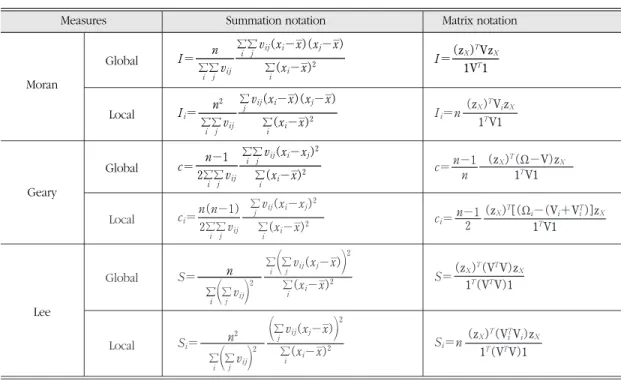
Table 1 lists three different univariate spatial association measures (global and local) not only in a summation notion but in a matrix notion.

The latter is crucial to define the measures compatible to the quadratic form.

A global spatial association measure should be defined as ratio of quadratic forms:

Г= (1)

where ∂ is a vector of deviants of a variable denoted by a vector of y, i.e., each value subtracted by mean, and T is a global spatial proximity matrix, a normalized form of a spatial weights matrix V. Equation (1) can be rewritten by utilizing a particular projection matrix that is defined as:

M₍₁₎=I- 11^T= (2)

This is a particular form of the projection matrix that projects a dependent variable and disturbances into a residual space that is

orthogonal to a design matrix X consisting of independent variables (Tiefelsdorf, 2000, 16).

That is,

M=I-X(X^TX)^-1X^T (3)

Since we focus on spatial association measures as pattern describers, the design matrix is solely composed of a vector of 1s resulting in (2). By utilizing (2), equation (1) is transformed to:

Г= (4)

where ∂=M(1)y and M₍₁₎ is an idempotent, symmetric matrix so that M(1)=M₍₁₎M₍₁₎.

Previous studies (Durbin and Watson, 1950;

1951; 1971; Henshaw, 1966; 1968) show that the distributional properties of a spatial association

y^TM₍₁₎TM₍₁₎y y^TM₍₁₎y 1

n

∂^TT∂

∂^T∂

Table 1. Univariate Spatial Association Measures

Measures Summation notation Matrix notation

Note: All the definitions of the local measures satisfy the additivity requirement that the average value of local measures is equal to the corresponding global measure.

Global Moran

Geary

Lee

Global Local

n Çi Ç

jvij

Çi Ç

j v_ij(x_i-x°)(xj-x°) Çi (xi-x°)²

I= (zX)^TVzX

1V^T1 I=

n² Çi Ç

jvij

Çjvij(xi-x°)(xj-x°) Çi (xi-x°)² Ii=

n-1 2Çi Ç

jvij

Çi Ç

jvij(xi-xj)² Çi (x_i-x°)² c=

n Çi {Ç

jv_ij}

2

Çi {Ç

jv_ij(x_j-x°)}² Çi (xi-x°)² S=

n-1 n

(zX)^T(„-V)zX

1^TV1 c=

n(n-1) 2Çi Ç

jvij

Çj vij(xi-xj)² Çi (xi-x°)²

c_i= n-1

2

(zX)^T[(„i-(Vi+Vi^T)]zX

1^TV1 ci=

(zX)^T(V^TV)zX

1^T(V^TV)1 S=

n² Çi {Ç

jvij}

2

{Çjvij(xj-x°)}² Çi (xi-x°)²

Si= (zX)^T(Vi^TVi)zX

1^T(V^TV)1 S_i=n

(zX)^TVizX

1^TV1 Ii=n

Local

Local Global

1- - … -

- 1- -

-_n¹ -¹_n … 1-¹_n

…

1 n 1

n 1 n

1 n 1

n 1 n

…

measure defined as in (4) are given by a matrix trace operation of M(1)TM₍₁₎under an assumption of independence among observations. Since a trace operation of matrix products is indifferent to the order of the product, computationally M₍₁₎TM₍₁₎ is reduced to M(1)T. When M₍₁₎T is denoted by K, first four central moments are given (Henshaw, 1966; 1968; Hepple, 1998;

Tiefelsdorf, 2000):

µ1=E(Г)= (5-1)

µ2=Var(Г)=2 (5-2)

µ3=8

(5-3) µ4=

{(n-1)³[4tr(K⁴)+tr(K²)²]

-2(n-1)²[8tr(K)tr(K³)+tr(K²)tr(K)²] +(n-1)[24tr(K²)tr(K)²+tr(K)⁴]

-12tr(K)⁴} (5-4)

In order to use equations above, T matrix (thus V matrix) should be symmetric. Skewness and kurtosis from the moments are given respectively by (Tiefelsdorf, 2000, 102):

∫1= (6-1)

∫2= (6-2)

This procedure also holds for local spatial association measures as long as they are defined a scale invariant ratio of quadratic forms as demonstrated for local Moran’s Ii (Tiefelsdorf, 1998; Boots and Tiefelsdorf, 2000).

Гi= (7)

T⁽ⁱ⁾ is a particular form of a local spatial proximity matrix derived from a global proximity matrix. Again, the matrix should be symmetric. As will be seen in the next section, spatial association measures are differentiated solely by the spatial proximity matrix.

2) Applications to univariate spatial association measures

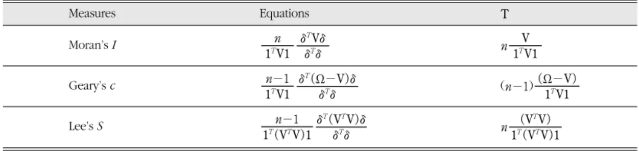
Table 2 summarizes the definition of the global spatial proximity matrix T for the three global univariate spatial association measures, Moran’s I, Geary’s c, and Lee’s S. Practically, a matrix of T is defined as a standardized form of a spatial weights matrix V. For example, when a row- standardized spatial weights matrix W is applied, T for Moran’s I becomes identical to V. Since T (thus V) should be symmetric in order to use equations (5-1)~(5-4), it may be necessary for some non-symmetric spatial weights matrices such as W to be transformed according to an equation:

(V+V^T) (8)

The „ matrix for Geary’s c should be further elaborated. According to Cliff and Ord (1981, 167), it is defined:

∑ii= Ç

j`(vij+vji) (9)

Simply the matrix is a diagonal matrix with row- sums when a spatial weight matrix is transformed symmetric.

Table 3 summarizes the definition of the local spatial proximity matrices T⁽ⁱ⁾for the three local univariate spatial association measures. A local

1 2 1 2

y^TM₍₁₎T⁽ⁱ⁾M₍₁₎y y^TM₍₁₎y

µ4

(µ2)²

12

(n-1)⁴(n+1)(n+3)(n+5)

{(n-1)²tr(K³)-3(n-1)tr(K)tr(K²)+2tr(K)³} (n-1)²(n+1)(n+3)

{(n-1)tr(K²)-tr(K)²} (n-1)²(n+1) tr(K)

n-1

µ3

(µ₂)³²

spatial weights matrix Vi is defined as a global spatial weights matrix whose elements are set to zeroes except for entries in ith row (Lee, 2008):

Vi= (10)

Even though Vidoes not have to be symmetric in calculating a local measure, it should be transformed symmetric in order to calculate distributional moments. When M(1)T⁽ⁱ⁾is denoted by K, the equations (5-1)~(5-4) compute first four moments at each location.

The local spatial weights matrix for local

Geary’s ci should be elaborated, because a local spatial proximity matrix cannot be directly derived from a global spatial proximity matrix

„-V. „i is a diagonal matrix of {vi1, …, vii, …, vin} with vii being added by Çjvij, a row-sum at each, Vi is defined according to equation (10), and diag() operation transforms a vector to a diagonal matrix. Thus, a local spatial weights matrix for Geary’s ciis given (Lee, 2008):

„i-(Vi+ViT)=

Table 2. Definitions of global spatial proximity matrix Tfor global spatial association measures

Measures Equations T

Moran’s I n

Geary’s c (n-1)

Lee’s S n (V^TV)

1^T(V^TV)1

∂^T(V^TV)∂

∂^T∂ n-1 1^T(V^TV)1

(„-V) 1^TV1

∂^T(„-V)∂

∂^T∂ n-1 1^TV1

V 1^TV1

∂^TV∂

∂^T∂ n 1^TV1

Table 3. Definitions of local spatial proximity matri T⁽ⁱ⁾ for local spatial association measures

Measures Matrix Notations

Moran’s Ii Equation

T⁽ⁱ⁾

Geary’s ci Equation

T⁽ⁱ⁾

Lee’s Si Equation

T⁽ⁱ⁾ n²(ViTVi) 1^T(V^TV)1

∂^T(ViTVi)∂

∂^T∂ n²

1^T(V^TV)1

[„i-(Vi+ViT)]

1^TV1 n(n-1)

2

∂^T[„i-(Vi+ViT)]∂

∂^T∂ n(n-1)

21^TV1 n²Vi

1^TV1

∂^TVi∂

∂^T∂ n² 1^TV1

(11) 0

vi1… vii … vin

0

vi1 0 -vi1

0 0

-vi1 … Çjvij-vii… -vin

0 0

-vin 0 vin

……

…

…

4. An Illustration

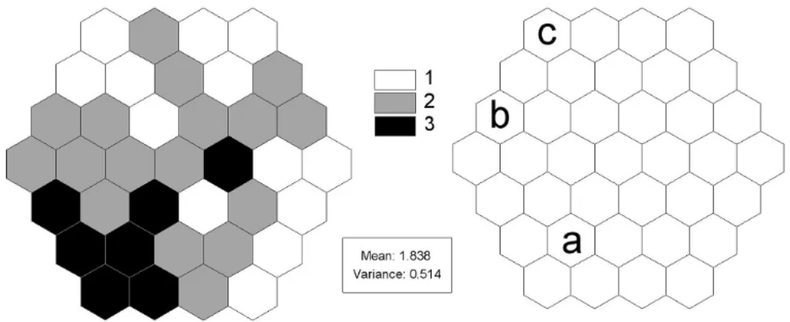
For an experiment, I designed a spatial pattern on a hypothetical space that is composed of 37 hexagons (Figure 1). The spatial pattern has a mean of 1.838 and a variance of 0.514. I choose three hexagons labeled respectively a, b, and c each of which has different linkage degrees (6 neighbors for a, 4 for b, and 3 for c) and different values (3 for a, 2 for b, and 1 for c). Two different spatial weights matrices are built; a binary connectivity matrix C for Moran’s and Geary’s measures, and a row-standardized and non-zero diagonal matrix W*, a row-standardized version of C*, ones on the diagonal of a binary contiguity matrix C for Lee’s measures.

Table 4 displays the distributional properties of the three global measures under the normality assumption. Moran’s I and Lee’s S are positively skewed while Geary’s c is negatively skewed.

The magnitude of skewness is not negligible for

Moran’s I and Lee’ S. The kurtosis of Lee’s S is relatively high. However, the normal approximation based on the first two moments is acceptable for all the three global measures particularly in situations where the sample size is large enough.

Table 5 reports the distributional properties of the three local measures under the normality assumption. There are several things noted from the table. First, the magnitude of variances are positively related to local linkage degrees at locations with C while negatively related with W*, which is correspondent to findings by Tiefelsdorf, et al. (1999). Second, Geary’s ci and Lee’s Si are positively skewed, while Moran’s Ii is negatively skewed. Third, the magnitude of skewness for Geary’s ci and Lee’s Si are not negligible at all.

Fourth, kurtosis for all the measures is extremely high, most prominent for Lee’s Si. All these things together dictate a restriction on the use of the normal approximation for local measures.

Figure 1. A hypothetical spatial pattern

Table 4. Distributional properties of global spatial association measures

Gloabl Measures Values Expectation Variance Skewness Kurtosis

Moran’s I 0.3092 -0.0278 0.0094 0.3362 3.1093

Geary’s c 0.6202 1 0.0123 -0.1289 2.9760

Lee’s S 0.4361 0.1560 0.0030 0.8011 3.8587

5. Concluding Remarks

The main objective of this paper was to formulate a generalized procedure to extract the first four moments of univariate spatial association measures for statistical testing under the normality assumption and to evaluate the viability of hypothesis testing based on the normal approximation for each of the spatial association measures. The main results are as follows. First, a generalized moment extraction procedure under the normality assumption was derived for both global and local measures.

When necessary matrices are defined in an appropriate way for each of the measures, the generalized method effectively yields the first four moments of sampling distribution. Second, the normal approximation based on the first two moments for the global measures turned out to be acceptable, while the notion did not appear to hold to the same extent for their local counterparts.

It should be noted that the procedure here can embrace any way of defining the spatial relationships among observations such that it is not bothered by a spatial proximity matrix with non-zero diagonal elements, which has been a fatal issue in the randomization approach as can

be seen from Lee (2004; 2008). The generalized procedure presented in this paper will most benefit those who obtain a spatial statistical measure but suffer from inability to offer the information on the distributional properties of the measure.

This study should be extended to utilize the higher moments. There might be several options.

First, the first three moments can be used to apply a Pearson Type III (gamma) function for a more reliable inferential test (Costanzo et al., 1983). With the first four moments (skewness and kurtosis), a beta distribution can be fitted for a nearly exact testing (Hepple, 1998).

References

Anselin, L., 1988, Spatial Econometrics: Methods and Models, Kluwer Academic Publishers, Boston.

Anselin, L., 1995, Local indicators of spatial association:

LISA, Geographical Analysis, 27(2), 93-115.

Boots, B.N. and Tiefelsdorf, M., 2000, Global and local spatial autocorrelation in bounded regular tessellations, Journal of Geographical Systems, 2(4), 319-348.

Cliff, A.D. and Ord, J.K., 1981, Spatial Processes: Models and Applications, Pion Limited, London.

Costanzo, M., Hubert, L.J., and Golledge, R.G., 1983, A Table 5. Distributional properties of local spatial association measures

Local Measures Locations Values Expectation Variance Skewness Kurtosis

a 2.3102 -0.0343 0.2097 -0.3819 7.4186

Moran’s Ii b -0.0228 -0.0228 0.1472 -0.3029 7.3852

c 0.5069 -0.0171 0.1137 -0.2587 7.3698

a 0.3889 1.2333 1.0007 2.1945 10.1688

Geary’s ci b 0.1945 0.8222 0.5248 2.1449 9.8645

c 0.1945 0.6167 0.3402 2.1393 9.7771

a 1.4938 0.1190 0.0261 2.5051 11.6792

Lee’s Si b 0.0028 0.1778 0.0582 2.5051 11.6792

c 0.6720 0.2292 0.0967 2.5051 11.6792

higher moment for spatial statistics, Geographical Analysis, 15(4), 347-351

Durbin, J. and Watson, G.S., 1950, Testing for serial correlation in least square regression. I, Biometrika, 37(3/4), 409-428.

Durbin, J. and Watson, G.S., 1951, Testing for serial correlation in least square regression. II, Biometrika, 38(1/2), 159-178.

Durbin, J. and Watson, G.S., 1971, Testing for serial correlation in least squares regression. III, Biometrika, 58(1), 1-19.

Henshaw, R.C., Jr., 1966, Testing single-equation least squares regression models for autocorrelated disturbances, Econometrica, 34(3), 646-660.

Henshaw, R.C., Jr., 1968, Errata: Testing single-equation least squares regression models for autocorrelated disturbances, Econometrica, 36(3/4), 626.

Hepple, L.W., 1998, Exact testing for spatial autocorrelation among regression residuals, Environment and Planning A, 30(1), 85-107.

Hubert, L.J., 1984, Statistical applications of linear assignment, Psychometrika, 49(4), 449-473.

Hubert, L.J., 1987, Assignment Methods in Combinatorial Data Analysis, Marcel Dekker, New York.

Lee, S.-I., 2001, Developing a bivariate spatial association measure: An Integration of Pearson’s r and Moran’s I, Journal of Geographical Systems, 3(4), 369-385.

Lee, S.-I., 2004, A generalized significance testing method for global measures of spatial association: An extension of the Mantel test, Environment and Planning A, 36(9), 1687-1703.

Lee, S.-I., 2008, A generalized randomization approach to local measures of spatial association, Geographical Analysis, forthcoming.

Leung, Y., Mei, C.-L., and Zhang, W.-X., 2003, Statistical test for local patterns of spatial association, Environment and Planning A, 35(4), 725-744.

Mielke, P.W., 1979, On asymptotic non-normality of null distributions of MRPP statistics, Communications in Statistics: Theory and Methods, A8(15) 1541- 1550; 1981, Erratum A10(17) 1795; 1982, Erratum 11(7) 847.

Rogerson, P.A., 2006, Statistical Methods for Geography:

A Student’s Guide, 2nd Edition, Sage Publications, London.

Siemiatycki, J., 1978, Mantel’s space-time clustering statistic: computing higher moments and a composition of various data transforms, Journal of Statistical Computation and Simulation, 7(1), 13-31.

Tiefelsdorf, M., 1998, Some practical applications of Moran’s I’s exact conditional distribution, Papers in Regional Science, 77(2), 101-129.

Tiefelsdorf, M., 2000, Modelling Spatial Processes: The Identification and Analysis of Spatial Relationships in Regression Residuals by Means of Moran’s I, Springer, Berlin.

Tiefelsdorf, M., 2002, The saddlepoint approximation of Moran’s I’s and local Moran’s Ii’s reference distributions and their numerical evaluation, Geographical Analysis, 34(2), 187-206.

Tiefelsdorf, M. and Boots, B., 1995, The exact distribution of Moran’s I, Environment and Planning A, 27(6), 985-999.

Tiefelsdorf, M., Griffith, D.A., and Boots, B., 1999, A variance-stabilizing coding scheme for spatial link matrices, Environment and Planning A, 31(1), 165-180.

Upton, G.J.G. and Fingleton, B., 1985, Spatial Data Analysis by Example: Volume 1 Point Pattern and Quantitative Data, John Wiley & Sons, New York.

Correspondence: Sang-Il Lee, Department of Geography Education, College of Education, Seoul National University, San 56-1, Sillim-dong, Gwanak-gu, Seoul 151-748, Korea (e-mail: [email protected], phone: +82-2-880-9028, fax: +82-2-882-9873)

교신: 이상일, 151-748, 서울특별시 관악구 신림동 산 56-1, 서 울대학교 사범대학 지리교육과(이메일: [email protected].

kr, 전화: 02-880-9028, 팩스: 02-882-9873)

Recieved June 13, 2008 Accepted June 25, 2008