• 검색 결과가 없습니다.

한국입자에어로졸학회

N/A
N/A
Protected

Academic year: 2021

Share "한국입자에어로졸학회"

Copied!
10
0
0

로드 중.... (전체 텍스트 보기)

전체 글

(1)

ISSN 2287-8130(Online) Particle and Aerosol Research

Part. Aerosol Res. Vol. 13, No. 4: December 2017 pp. 173-182 http://dx.doi.org/10.11629/jpaar.2017.12.30.173

발전소 굴뚝에서의 입자 분산에 대한 수치해석

심 정 보1)⋅유 동 현1)*

1)

포항공과대학교 기계공학과

(2017년 11월 17일 투고, 2017년 12월 5일 수정, 2017년 12월 8일 게재확정)

Numerical study of particle dispersion from a power plant chimney

Jeongbo Shim

1)

, Donghyun You

1)*

1)

Department of Mechanical Engineering, POSTECH

(Received 17 November 2017; Revised 5 December 2017; Accepted 8 December 2017)

Abstract

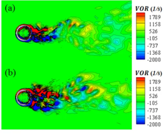
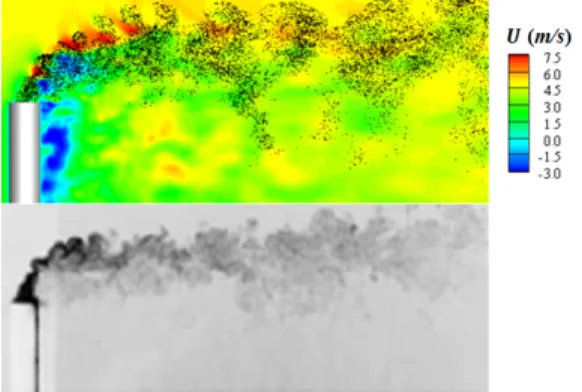
An Eulerian-Lagrangin approach is used to compute particle dispersion from a power plant chimney. For air flow, three-dimensional incompressible filtered Navier-Stokes equations are solved with a subgrid-scale model by integrating the Newton's equation, while the dispersed phase is solved in a Lagrangian framework. The velocity ratios between crossflow and a jet of 0.455 and 0.727 are considered. Flow fields and particle distribution of both cases are evaluated and compared. When the velocity ratio is 0.455, it demonstrates a Kelvin-Helmholtz vortex structure above the chimney caused by the interaction between crossflow and a jet, whereas the other case shows flow structures at the top of the chimney collapsed by fast crossflow. Also, complex wake structures cause different particle distributions behind the chimney. The case with the velocity ratio of 0.727 demonstrates strong particle concentration at the vortical region, whereas the case with the velocity ratio of 0.455 shows more dispersive particle distribution. The simulation result shows similar tendency to the experimental result.

Keywords: particle-laden flow, power plant chimney, Eulerian-Lagrangian method, large-eddy simulation

* Corresponding author.

Tel:+82-54-279-2191

E-mail:[email protected]

(2)

1. Introduction

Since industrialization, creating pollutants and harmful particles from burning fossil fuel has been inevitable.

The most critical concern of the air pollution is the condition of the air that people inhale. Those pollutants are usually particles that are resultant of burning fossil fuel in various environment, such as power plant industries, fossil-fuel-burning vehicles, and so on.

These particles have a wide spectrum in size from submicrometers to a couple of hundred micrometers.

Resultant particles, especially those that are smaller than 10 micrometers, can harm people's health.

These small sized particles can critically damage human beings; people who are exposed to fine particles over a long period of time are likely to have more heart and lung problems than those who are not.

According to the report by Centers for Disease Control and Prevention, it is evident that the risk of heart disease death can be reduced by 15% with a decrease of 10  of 2.5  or smaller particulate matters in every cubic meter (Centers for Disease Control and Prevention, 2013). In order to evaluate particle concentration within air, understanding the interaction between particles and flow is crucial. Especially, understanding the flow characteristics and particle motions within flow in certain environments where pollutants are injected and dispersed are critical such as the power plant chimney. By evaluating particle distribution in that environment, it is possible to keep track of particle concentration at specific locations.

A jet injecting from an external cylinder in crossflow has been investigated by many researchers and analyzed with its flow characteristics. Patankar et al. (1977), one of the early research groups, explored flow characteristics in a round turbulent jet deflected by crossflow using Reynolds Average Navier-Stokes (RANS) equations with a two equation model. They investigated flow characteristics and statistics in various velocity ratios between a free stream and a jet.

Sykes et al. (1986) also studied on the vorticitiy dynamics of the jet in crossflow. This study investigated

the effect of various diameters of a round jet. They found out variations in vorticity dynamics when the velocity ratios between the jet, 



, and crossflow,

, are different range from 

 



  to

 



  . For small velocity ratios, 

 



≦  , the three-dimensional wrapping process alters the initial form of azimuthal vorticity, whereas the large velocity ratio, 

 



  , causes azimuthal vortices to follow flow structures created by crossflow and a cylinder.

Unlike other investigations on a jet in crossflow, there exists only a little research in a particle-laden jet when crossflow is present. Saïd et al. (2005) carried out experimental and numerical studies to investigate pollutant dispersion from a chimney. They injected glycerin particles from a chimney in crossflow and visualized flow characteristics and particle dispersion with various velocity ratios between crossflow and a jet. They also numerically investigated flow around a cylinder with a RANS solver, when the jet is injected.

They found out there is an instability region created at the interface between a jet and crossflow. Diez and Torregrosa (2011) performed an experimental investigation on a particle-laden jet with crossflow, and evaluated particle dispersion and flow characteristics. They analyzed the effect of the particle-laden jet by comparing with an unladen jet. According to Diez and Torregrosa, particles tend to enhance turbulent dissipation downstream of the test section. Also, they perform the experiments with two different Stokes numbers,  ×

 

and 0.24, and evaluated particle distribution with corresponding Stokes number.

There are many studies that show flow characteristics in a jet from an extended cylinder when crossflow is present. Flow characteristics of a jet in crossflow have been numerically and experimentally investigated in detail (Patankar et al., 1977, Sykes et al., 1986).

However, it seems there are not enough studies that

computationally evaluate particle motions and

distribution in the case where a particle-laden jet from

the extended cylinder interacts with crossflow in an

(3)

unsteady domain. In the present study, an Eulerian- Lagrangian method is used to investigate unsteady flow characteristics and corresponding particle motions in order to figure out particle distribution around the power plant chimney.

2. Numerical methods

In the present study, an Eulerian-Lagrangian method is employed to numerically evaluate the flow characteristics and corresponding particle distribution.

The Eulerian-Lagrangian method is described here briefly. For Eulerian solver, finite-volume-based large-eddy simulation (LES) is used to investigate unsteady flow characteristics of air around the chimney. The discrete phase is computed in a Lagrangian framework in order to figure out particle distribution caused by flow motions in the jet in crossflow. Two methods are coupled in one-way where only the gaseous phase affects the particle phase.

2.1 Gaseous phase

In the gaseous phase, three-dimensional incompressible filtered Navier-Stokes equations are solved on unstructured grids. LES method is used to solve governing equations in a time-marching domain.

Equations are written as

 

 

  (1)

 

 

  

 

 

  

 

   

 

  



 

  





 (2)

where 

represents flow velocity, P indicates pressure,

indicates spatial coordinates, 



  

  

 

indicates an anisotropic part of the sub-grid scale stress tensor, the subscript indicates directions in three-dimensional Cartesian coordinates and the overbar represents filtered variables. In this computation, dynamic Smagorinsky model is employed in order to

capture the spatial and temporal variation of turbulent characteristics (Germano et al., 1991). Momentum equations are non-dimensionalized by the reference length, velocity and density. The reference Reynolds number is defined as  

 

 

 

 

 



 

where

 

, 

 

, 

 

and 

 

indicate the reference density, length, velocity and viscosity, respectively. In the present study, in-house code is used to solve fluid flow. Second-order central-difference scheme is used in space and Crank-Nicolson scheme is used in time.

2.2 Particle phase

The governing equations for the particle motion are based on Basset-Boussinesq-Oseen equation (Crowe et al., 1998). There are a few assumptions to be made for the equations of the particle phase. They are:

1. Particles are perfect spheres

2. Density ratio between the particle and the fluid is bigger than 

.

3. Particle size is very small compared to the Kolmogorov length scale.

4. Interaction between particles can be neglected.

Therefore, the Lagrangian equations for particles are written as follows:

 



 

 , (3)

 



   

 



 

 (4)

where 

indicates the particle location, 



represents the velocity of the fluid at the particle location,  indicates the drag coefficient and  

is the Stokes number. The drag coefficient and the Stokes number can be defined as

      

 (5)

 

  

  

 

 

 

(6)

where  

represents particle Reynolds number which

(4)

is defined as 

 

 





 

 , 

indicates the particle characteristic time scale, 

represents the characteristic time scale of flow, 

indicates the particle density and

indicates the particle diameter.  

is the Stokes number which is defined as the ratio of the characteristic time of a particle to a characteristic time of the flow. The drag coefficient is within 5%

deviation from the standard drag curve where constants

 and  are 0.15 and 0.687, respectively. In this simulation, the effect of the gravitational force is neglected because sizes of most particles are less than 5  . For the particle solver, in-house code is used. A third-order Runge-Kutta time-stepping algorithm is employed for integration of the governing equations.

2.3 Computational domain and boundary conditions

Fig. 1. Schematic of a computational domain

The schematic of the computation domain for the present study is shown in Fig. 1. Crossflow is blown

at the inlet of the domain. The streamwise, normal and spanwise directions are set as x, y and z, respectively.

There is a wall-mounted cylinder located at the origin of the coordinates and a particle-laden jet is injected at the entry of the chimney. The size of the domain is non-dimensionalized with the diameter  and the height

 of the chimney and it is  in the streamwise direction,  in the normal direction and  in the spanwise direction. Totally 8 million hexahedral computational cells are used to construct the domain.

Fig. 2 shows the top view of computational grids at

   . An O-type grid topology is used to construct computational cells around the cylinder in order to maximize grid quality.

Fig. 2. Computational grids at    in an XZ-plane

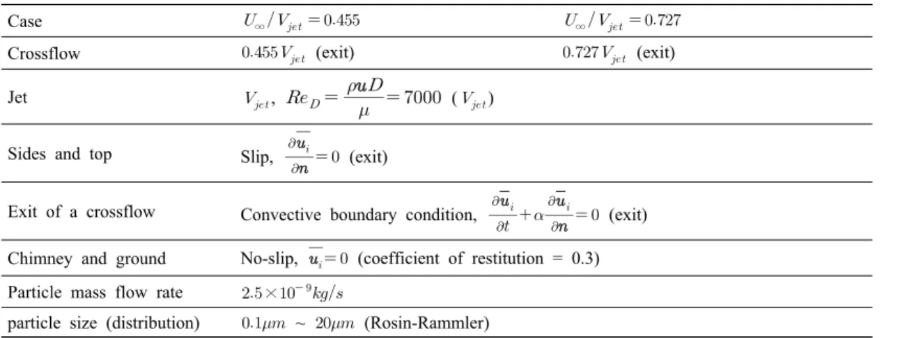
Boundary conditions for the present study are summarized in Table 1. For the top and side boundary conditions of the continuous phase, slip boundary

Case 

 



  

 



 

Crossflow 



(exit)  



(exit)

Jet 



, 

 



 

(



)

Sides and top Slip,



 

  (exit)

Exit of a crossflow Convective boundary condition,



 

  

 

  (exit)

Chimney and ground No-slip,

  (coefficient of restitution = 0.3) Particle mass flow rate  ×

 



particle size (distribution)  ~  (Rosin-Rammler)

Table 1. Boundary conditions for flow (particle)

(5)

conditions are used, while exit boundary conditions, which particles are destroyed, are used for the discrete phase. For the surface of a hollow cylinder and the ground, no-slip boundary conditions are used for the continuous phase, while wall-bounded boundary conditions with restitution of coefficient valued as 0.3 are used for particles. At the exit of crossflow, the convective boundary condition is used for the continuous phase. Two inlet velocities of crossflow,

, and a constant jet velocity, 



 11 m/s, are used. Flow velocity is normalized with the corresponding jet velocity, 



. For the crossflow boundary condition, the experimental velocity profile by Saïd et al. (2005) is used in the case of

 



  with turbulent intensity of 0.2%. The velocity profile of 

 



  in the boundary layer was projected to the boundary layer velocity profile of 

 



  .

The projected velocity profile in the boundary layer was calculated by multiplying velocity ratio between two crossflow of 

 



  and 

 



 

and those profiles are shown in Fig. 3. Two cases,

 



  and 

 



  , are selected and compared in order to figure out impacts of different flow characteristics on particle distribution. The mean velocity profile at the entry of the chimney shown in Fig. 4 comes from the Direct Numerical Simulation (DNS) result at     (Eggels et al., 1994). The X-axis represents the radius normalized with the pipe

diameter and the Y-axis represents velocity normalized with the maximum velocity of a pipe. Turbulent intensity of 0.2% is used for the velocity at the entry of the chimney. For the discrete phase, particles are injected with flow velocities at the entry of the chimney. The size of particles is distributed from

 to  with Rosin-Rammler distribution.

Rosin-Rammler distribution has the mean diameter as

 and the spread parameter as 1.5. For material properties, the fluid is assumed as air with the density of 

and the kinematic viscosity of

 ×

 

 and particles are assumed as glycerin particles with the density of  ×



as in the experiment (Saïd et al., 2005).

Particles are injected from the entry of the chimney when the flow field is statistically converged. In order to get statistically converged flow field, the flow from the inlet of crossflow has to go through several passage times. Therefore, the injected time for particles are different for both cases. The injected times for particles are about 0.7s in the case of 

 



 

and 0.65s in the case of 

 



  . Also,

 ×

 

 is selected to be the time step for flow and the total integration time step for particles because the selected time step is less than the Courant- Friedrichs-Lewy (CFL) condition value of 1 and able to capture particle path. The total run time for the present study is about 1s for both cases.

Fig. 3. Velocity profiles at the entry of crossflow (Saïd et al. , 2005)

Fig. 4. Velocity profile at the entry of a chimney

(Eggels et al. , 1994)

(6)

3. Results and discussion

3.1 Flow field

Fig. 5. Mean streamwise velocity at    in an XY-plane (a) 

 



  (b) 

 



 

Fig. 6. Instantaneous streamwise velocity near the exit of a chimney at    in an XY-plane (a) 

 



  (b) 

 



 

Flow characteristics of the two cases, 

 



 

and 

 



  , are compared. First of all, mean flow fields in an XY-plane for the case of

 



  and 

 



  are compared in Fig. 5. For both cases, flow from the chimney is quickly affected by streamwise crossflow. Also, bending angles, the angles between the bending jets and ground, caused by the interaction between crossflow and the jet are visible. The bending angle in the case of 



  , approximately 55° from the top of the chimney, is smaller than that of the case of 

 



  , approximately 45°. Furthermore, flow passing the chimney tends to have negative values at the rear part of the chimney which indicates creation of strong vortices.

In order to evaluate unsteady flow characteristics, Fig. 6 shows the instantaneous streamwise velocity near the exit of the chimney in an XY-plane. Both

instantaneous contours in Fig. 6 show the instability interface between crossflow and the jet. This instability region is created because there is velocity shear caused by a velocity difference between two fluids. The instability creates patterned bubble-like structures at the top of the chimney in the case of 

 



  , whereas the flow structures in the case of

 



  are small in size and more chaotic.

Also, bubble-like structures for the case of

 



  tend to be located at higher positions which indicate bigger influence of the jet on the free stream.

Influence of the jet on crossflow can be shown in Fig. 7, where contours of the mean normal velocity of two cases in an XY-plane are shown. In the case of

 



  , the jet reaches higher position than that of the other case. It is evident that influence of the jet to the free stream is bigger in the case of

 



  . However, the size of the jet-influencing zone is narrower in the case of 

 



  . This interesting phenomenon can be seen in Fig. 8 which shows the instantaneous normal velocity above the chimney. For the case of 

 



  , the bubble- like flow structures above the chimney show unique patterns. The jet coming out of the chimney breaks into small parts and creates bubbles, whereas the flow structures in the case of 

 



  collapse together.

Fig. 7. Mean normal velocity at    in an XY-plane

(a) 

 



  (b) 

 



 

(7)

Bubble structures in the velocity fields can be evaluated by analyzing vorticity fields. Vorticity of two cases are shown in an XY-plane to analyze unsteady physics of flow in Fig. 9. Just like the instantaneous velocity fields, the spanwise vorticity in the case of

 



  shows jet breakup which creates organized spanwise vortices at the top of the chimney.

On the other hand, vortices in the case of

 



  lose structures. Also, vortices of the second case tend to last longer as they flow downstream. These phenomena can be explained with contours in Fig. 10. Fig. 10 shows turbulent kinetic energy for both cases in an XY-plane. Turbulent kinetic energy in the case of 



  quickly dissipates whereas turbulent kinetic energy in the case of 

 



  lasts longer. This explains that stronger fluctuation results long-lasting unsteady flow characteristics.

Fig. 8. Instantaneous normal velocity near the exit of a chimney at    in an XY-plane

(a) 

 



  (b) 

 



 

Fig. 9. Z-vorticity in an XY-plane at    (a) 

 



  (b) 

 



 

Fig. 10. Turbulent kinetic energy at    in an XY-plane (a) 

 



  (b) 

 



 

Fig. 11. Mean streamwise velocity at    in an XZ-plane (a) 

 



  (b) 

 



 

For different perspectives, analysis of flow fields in a different plane has been carried out. Fig. 11 shows mean streamwise velocity contours of two cases at

   in an XZ-plane. Two contours show stagnation points and separation points of flow in both cases. Fig.

12, contours of vorticity in an XZ-plane, demonstrates unsteady nature of flow structures at the top of the chimney. The contour for the case of 

 



 

describes patterned flow structures of vortices. In

contrast, vortices in the case of 

 



  show

collapsed wake pattern. This is because the jet bending

caused by faster crossflow heavily influences the flow

patterns. As a result, flow patterns are distorted and

eventually break down into small parts. Therefore, the

size of spanwise vortices for the second case becomes

smaller behind the chimney.

(8)

Fig. 12. Y-vorticity at    in an XZ-plane (a) 

 



  (b) 

 



 

Fig. 13. Turbulent kinetic energy at    in an XZ-plane (a) 

 



  (b) 

 



 

Not only the size of vortices is different between two cases, but the width of wakes behind the chimney is also different. In Fig. 12, the width of wakes in the case of 



  tends to be narrower at the rear of the chimney. However, as vortices travel downstream, a group of wakes tends to be and patterned dispersed in spanwise direction. On the other hand, the width of wakes behind the chimney seems to have constant thickness and show more chaotic structures. This unique unsteady structure of flow can be explained with turbulent kinetic energy contours shown in Fig. 13. In Fig. 13, stronger turbulent kinetic energy encourages more chaotic motions of flow in the case of 

 



  . However, the contour in the case of 

 



  shows smaller turbulent kinetic

energy which results organized flow structures.

3.2 Particle distribution

Unique flow structures in both cases cause different particle distribution when velocity ratios are different.

Particle distribution with streamwise velocity contours at  ≥  in an XY-plane is shown in Fig. 14. There are some common features between two cases. Both cases show that particles tend to follow vortical structure created by interaction between the jet and crossflow. Also, as particles flow downstream, they are vertically dispersive.

Fig. 14. Particle distribution at  ≥  in an XY-plane (a) 

 



  (b) 

 



 

However, the level of vertical dispersion is different.

Most particles tend to be located at      as they are initially injected from the chimney. As they flow downstream, they tend to be vertically dispersed in the region      in the case of

 



  . On the other hand, particles in the case of 

 



  are vertically less dispersive.

Most particles are concentrated in the region where

     as they are injected into the main stream.

At the downstream of the domain, they tend to be located in the region where      . Difference in the level of dispersion can be explained by intensity of vorticity throughout the domain. Unlike the case of

 



  , vortical structures tend to be quickly

dissipated at the downstream of the domain in the case

of 



  shown in Fig. 9. Therefore, flow

(9)

no longer has coherent structures to keep particles being segregated within vortices. As a result, particles are vertically less dispersive in the case with long-lasting vortical structures.

Also, difference in particle dispersion can be found when particles are injected from the chimney. In the case of 

 



  , particles tend to be concentrated in bubbles created in the region of instability which shows particles following the Kelvin-Helmholtz instability. However, particles in the other case do not describe the region of instability because strong crossflow crumbles flow structures. As a result, particles tend to follow the bulk stream of the jet.

Fig. 15. Particle distribution at  ≥  in an XZ-plane (a) 

 



  (b) 

 



 

Particle distribution seen from an XZ-plane is shown in Fig. 15. In the case of 

 



  , particles follow y-vortices as they travel. Most particles tend to be concentrated behind the cylinder where    . In contrast to the first case, particles more dynamically follow wakes and be patterned behind the cylinder in the case of 

 



  . Difference in particle distribution in both cases can be explained by turbulent length scale. In the case of 



  , a relatively slow crossflow causes bigger flow length/

time scales which lead small particles to follow the bulk stream. On the other hand, flow with smaller scales make particles to be able to correspond to their

comparative scales. As a result, particles in the case of

 



  are able to follow smaller flow structures.

Lastly, the present computational results are compared to the experimental result carried out Saïd et al. (2005) in Fig. 16. The case of 

 



  is selected to be compared to the experimental result of

 



  . Unfortunately, the crossflow velocity profile data in the case of 

 



  do not exist. Therefore, the following case of 

 



 

is selected to be compared because the case has the close velocity ratio to that of the experiment. The following simulation case well describes the Kelvin- Helmholtz instabilities above the chimney as well as particle distribution throughout the domain. Even though the velocity ratios between two cases are slightly different, the overall result of the simulation case shows similar tendency to that of the experimental result.

Fig. 16. Comparison between the present simulation for the case of 

 



  and the experiment for the case of 

 



 

( Saïd et al ., 2005)

4. Conclusion

In the present study, two cases, 



  and

 



  , are computed with an Eulerian-Lagrangian

approach. By using LES, evaluation of unsteady flow

(10)

fields and particle distribution is carried out. Both cases demonstrate distinguishable flow structures and characteristics as well as interesting particle distribution throughout the computational domain.

The flow field above the chimney shows the unique nature caused by interaction between crossflow and the jet. Even though flow from the chimney dominates the flow structure for both cases, level of influence is different. When the jet heavily influences the flow field of crossflow, the region of strong instability, Kelvin-Helmholtz instability, is depicted. On the other hand, the influence of crossflow has been increased for the case of 

 



  which results the collapse of flow structures.

Vortical structures for both cases are also compared.

Vortical structures last longer in the case of

 



  due to heavy fluctuation of the flow field throughout the domain. This unsteady nature of flow results different particle distribution in both cases.

The first case when the velocity ratio is

 



  , particles tend to follow the instability region. However, as they march toward the downstream, they tend to be less responsive to corresponding flow structures. On the other hand, the case of 



  demonstrates strong particle concentration at the downstream. Also, one of the computational results is compared with the experimental result. The result of the present study shows similar tendency to the experimental result.

5. Acknowledgement

This study was supported bythe Korea Institute of Energy Technology Evaluation and Planning (KETEP) and the Ministry of Trade, Industry and Energy (MOTIE) of the Republic of Korea (No. 20161110100230).

6. References

Centers for Disease Control and Prevention (2013). Health impacts of fine particles in air. Retrieved from https://ephtracking.cdc.gov/showAirHIA.action.

Crowe, C. T., Sommerfeld, M., & Tsuji, Y. (1998).

Fundamentals of gas-particle and gas-droplet flows. Boca Raton, FL: CRC Press.

Diez, F. J., Torregrosa, M. M., & Pothos, S. (2011). A comparison between round turbulent jets and par- ticle-laden jets in crossflow by using time-re- solved stereoscopic particle image velocimetry.

Journal of Fluids Engineering, 133(9), 091301.

Eggels, J. G. M., Unger, F., Weiss, M. H., Westerweel, J., Adrian, R. J., Friedrich, R., & Nieuwstadt, F. T. M. (1994). Fully developed turbulent pipe flow: a comparison between direct numerical sim- ulation and experiment. Journal of Fluid Mechanics, 268, 175-210.

Germano, M., Piomelli, U., Moin, P., & Cabot, W. H.

(1991). A dynamic subgrid‐scale eddy viscosity model. Physics of Fluids A: Fluid Dynamics, 3(7), 1760-1765.

Patankar, S. V., Basu, D. K., & Alpay, S. A. (1977).

Prediction of the three-dimensional velocity field of a deflected turbulent jet. Journal of Fluids Engineering, 99(4), 758-762.

Saïd, N. M., Mhiri, H., Le Palec, G., & Bournot, P. (2005).

Experimental and numerical analysis of pollutant dispersion from a chimney. Atmospheric Environment, 39(9), 1727-1738.

Sykes, R. I., Lewellen, W. S., & Parker, S. F. (1986).

On the vorticity dynamics of a turbulent jet in

a crossflow. Journal of Fluid Mechanics, 168,

393-413.

수치

Fig.  2.  Computational  grids  at      in  an  XZ-plane
Fig.  3.  Velocity  profiles  at  the  entry  of  crossflow  (Saïd   et  al. ,  2005)
Fig.  6.  Instantaneous  streamwise  velocity  near  the  exit  of  a  chimney  at      in  an  XY-plane  (a)   ∞       (b)   ∞     
Fig.  9.  Z-vorticity  in  an  XY-plane  at      (a)   ∞       (b)   ∞     
+3

참조

관련 문서

The present study used the guinea pig CPI model to investigate the effect of hypoxia on the development of mature neurons and to evaluate the relationship

 Action causing unsteady flow takes place over a period of many 2 L/a time intervals, then it would be more appropriate to use rigid water column theory..  On the

~ In steady flow, Lagrangian path lines are the same as the Eulerian streamlines, and both are the same as the streak lines, because the streamlines are then fixed in space

~ In steady flow, Lagrangian path lines are the same as the Eulerian streamlines, and both are the same as the streak lines, because the streamlines are then fixed in space

The following study qualitatively and quantitatively investigated and analyzed North Korea’s chemistry textbook’s contents and activities in order to

The purpose of this study is to present the background, necessity and purpose of the study in Chapter 1, and the second part of the theoretical study is related to the

It is to trace the period of their appearances and changes and also to illuminate coinage characteristics and method of architectural terminology used

In this study, water flow system of Danghang Bay, which has the narrow and long topographical characteristics with the narrow bay mouth and its flow