유도전동기의 고장 진단을 위한 효과적인 특징 추출 방법
1)흥 뉘엔*, 김종면*
An Effective Feature Extraction Method for Fault Diagnosis of Induction Motors
Hung Nguyen*, Jong-Myon Kim*
요 약
본 논문은 고장 분류 시스템을 위해 진동 신호로부터 특징 벡터를 자동적으로 추출하는 효과적인 기법을 제안한 다. 기존의 멜-주파수 캡스트럼 계수는 진동신호의 노이즈에 민감하여 분류 정확도를 감소시키는 단점이 있다. 이 러한 문제를 해결하기 위해 본 논문은 4단계 필터 뱅크로 구성된 스펙트럴 엔벨로프 캡스트럼 계수 분석을 제안하 며, 4단계는 (1) 모든 진동 신호의 스펙트럴 엔벨로프를 기술하기 위한 선형 예측 코딩 알고리즘 사용 단계, (2) 일반적인 스펙트럴 모양을 얻기 위해 모든 엔벨로프의 평균화 단계, (3) 평균 엔벨로프와 그 주파수의 최대값을 찾 기 위한 기울기 하강 방법 사용 단계, (4) 엔벨로프의 주파수 사이의 거리로부터 계산된 중앙값을 얻는데 사용되는 비 중첩 필터 뱅크 단계로 구성된다. 이 4-단계 필터 뱅크는 특징 벡터를 추출하기 위해 캡스트럼 계수 계산에 사용 된다. 마지막으로 유도전동기의 결함 형태를 구분하기 위해 이러한 특수 파라미터를 사용하는 다중 계층 서포트 벡 터 머신을 사용한다. 모의실험 결과, 제안하는 방법은 약 99.65%의 분류 성능을 보이며, 동시에 기존 방법들보다 우수한 성능을 보인다.
▸Keywords : 고장 분류, 특징 추출, 캡스트럼 계수, 서포트 벡터 머신
Abstract
This paper proposes an effective technique that is used to automatically extract feature vectors from vibration signals for fault classification systems. Conventional mel-frequency cepstral coefficients (MFCCs) are sensitive to noise of vibration signals, degrading classification accuracy.
To solve this problem, this paper proposes spectral envelope cepstral coefficients (SECC) analysis, where a 4-step filter bank based on spectral envelopes of vibration signals is used: (1) a linear
∙제1저자 : Hung N. Nguyen ∙교신저자 : 김종면
∙투고일 : 2012. 10. 31, 심사일 : 2012. 12. 10, 게재확정일 : 2013. 1. 1.
* 울산대학교 전기공학부(School of Electrical Engineering, University of Ulsan)
※ This work was supported by Basic Science Research Program through the National Research Foundation of Korea(NRF) funded by the Ministry of Education, Science and Technology(No. 2012R1A1A2043644).
predictive coding (LPC) algorithm is used to specify spectral envelopes of all faulty vibration signals, (2) all envelopes are averaged to get general spectral shape, (3) a gradient descent method is used to find extremes of the average envelope and its frequencies, (4) a non-overlapped filter is used to have centers calculated from distances between valley frequencies of the envelope.
This 4-step filter bank is then used in cepstral coefficients computation to extract feature vectors.
Finally, a multi-layer support vector machine (MLSVM) with various sigma values uses these special parameters to identify faulty types of induction motors. Experimental results indicate that the proposed extraction method outperforms other feature extraction algorithms, yielding more than about 99.65% of classification accuracy.
▸Keywords : fault classification, feature extraction, cepstral coefficients, support vector machines
I. 서 론
Induction motors are essential components in many industrial processes which deal with moving and lifting products. However, unexpected machinery failure results in loss of production, high emergency maintenance costs, and expected process downtime [1]. Thus, early fault diagnosis techniques can increase the safety of motor operations, reduce emergency maintenance costs, and minimize downtime [1-3].
The key challenge of the fault detection and classification system of induction motors is the improvement of diagnostic accuracy based on a given amount of information which is usually contaminated by white or colored noise in industrial environments.
Many researchers have mainly utilized current and voltage as system inputs of the fault detection system because they are easy to measure. In spite of having non-stationary and non-deterministic characteristics, vibration signals are also widely used for fault diagnosis systems because vibration signals often direct link to the status of machines [4]. Thus, vibration monitoring is the most reliable and effective method to detect whether the machinery system is healthy or not [5].
Generally, there are two main steps in a typical fault diagnosis system: (1) features generation which encodes the classification information in a more compact way compared with original acquired signals and (2) pattern classification based on the feature vectors obtained from the first step. Feature extraction is an important step in designing any kinds of classification systems because classification accuracy highly depends on the features which are used as an input of a classifier. In addition, selecting the proper number of features is important because it help to avoid overfitting to the specific training dataset and design classifiers.
Vibration signals have been analyzed in time domain, frequency domain, or both the time-frequency domain to generate feature vectors [6-9]. Many researchers extracted the statistical values (e.g., mean, variance, root-mean-square, and kurtosis) or spectral power coefficients from the time and frequency analysis [6, 8, 9]. These features were well-suited for most mechanical systems. For instance, short-time Fourier transform (STFT), discrete wavelet transform (DWT), and mel-frequency cepstral coefficients (MFCCs) were often used to extract the spectral coefficients [6, 8, 10-12]. Yang et al. [13, 14] utilized aforementioned features which were extracted from both time and frequency domain for rotating machinery and
cavitations of a butterfly valve.
In the feature-based diagnostic process, a huge dimensionality problem of features can possibly occur after feature extraction. This cannot be avoided because all of the features are not useful in the classification task. The existence of irrelevant features tends to degrade the performance of the classifier. To reduce or select an optimal number of features, several methods have been introduced, such as principal component analysis (PCA) [15], independence component analysis (ICA) [16], and singular values decompositions [23].
There are two main classifier models for fault classification: analytical model based methods and artificial intelligence (AI) based methods (e.g., knowledge based models and data based models) [17-19]. Although analytical and knowledge-based models are effective for fault classification, they provide poor classification performance of induction motors because of lacking adaptability and the random nature of vibration signals [19]. Thus, Data-based models have been used for fault classification of induction motors, such as neural networks, fuzzy systems, and support vector machines (SVM). In this paper, we employ SVM as a classifier due to the highest generalization performance when the number of training samples is limited. In addition, we utilize the standard deviation (σ) values of the Gaussian radial basic kernel function of SVM because they supports a strong effect on the classification accuracy, which in turn affects system performance [20].
For feature extraction, MFCCs have been widely used [6. 8, 10-12], but they are sensitive to noise, which degrades classification accuracy. To solve this problem, this paper proposes a robust feature extraction method, called spectral envelope cepstral coefficients analysis (SECC), where a 4-step filter bank based on spectral envelopes is used: (1) a linear predictive coding (LPC) algorithm to specify spectral envelopes of all faulty vibration signals, (2) averaging all envelopes to get general spectral
shape, (3) a gradient descent method to find maxima and minima of the average envelope and its frequencies, (4) a non-overlapped filter bank to have centers calculated from distances between valley frequencies of the envelope. This filter bank is then used in cepstral coefficients computation to generate feature vectors. Finally, we utilize multi-layer support vector machines (MLSVM) to classify several faults of induction motors. In addition, different values of σ are evaluated in order to investigate the impact of the sigma value on classification performance.
The rest of this paper is organized as follows.
Section 2 discusses cepstral coefficient analysis and support vector machines. Section 3 presents the proposed fault classification system with new frequency scale and multi-layer support vector machine for multi-class problems. Section 4 describes the impact of various sigma values on the classification performance for both noise and noise-free vibration signals, and Section 5 concludes this paper.
II. Background Information
1. Cepstral Coefficients Analysis
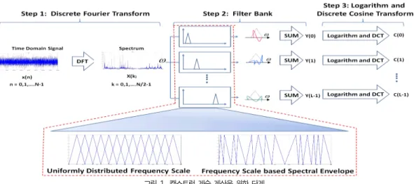
Cepstral coefficients analysis (CCA) with mel frequency scale has been widely used in the field of speech recognition because it is able to handle dynamic features of speech by extracting both linear and non-linear signal properties. Thus, CCA can be effective in extracting features of vibration signals since vibration signals also contain both linear and non-linear features. Fig. 1 shows the concise steps involved in the computation of the cepstral coefficients [10, 22].
Step 1: Use the fast Fourier transform (FFT) of vibration signals by using:
그림 1. 캡스트럼 계수 계산을 위한 단계
Fig. 1. The procedure for the cepstral coefficients computation
1 2
0
( ) 1 ( ) ( ) ,
N j m n
F n
Y m x n n e
N
p
w
- -
=
= å (1)
where N is the number of points used to calculate the discrete Fourier transform (DFT), 0≦n≦N-1, and w(n) is the Hamming window function given by:
( ) (0.5 0.5 cos 2 ), 1 n n
N w =b - p
- (2)
where 0≦n≦N-1 and β is the normalized factor in which the root mean square of the window is unity [22].
Step 2: Multiply the power spectrum by each filter in the filter bank, which has a triangular band pass frequency response whose magnitude is determined by (3)
0 ( ) ( 1) ( ) ( 1)
( 1) ( ) ( ) ( ) ( 1)
( , )
( ) ( 1)
( ) ( ) ( 1) ( ) ( 1)
0
c
c
c c
c c
c
c c
c c
for f k f m f k f m
for f m f k f m f m f m
H k m
f k f m
for f m f k f m f m f m
for
< -
- -
- £ <
- -
= - +
£ < +
- +
,
( ) c( 1) f k f m ì
ï ï ïï í ï ï
ï ³ +
ïî
(3)
where fc is the cut-off frequency of each filter, m indicates the order of filter in the filter bank, and k
ranges from 0 to fs/2 in which fs is the sampling rate.
Step 3: Convert the logarithmic spectrum back to the time domain. This conversion is achieved by taking the DCT of the spectrum such as:
1
10 0
cos( ( 0.5)) log ( ),
N i
m n
n
C m n Y
N
- p
=
=å + (4)
where 0≦m≦N-1, and L is the number of cepstral coefficients extracted from the vibration signal.
These coefficients are then used as feature vectors of the vibration signal.
2. Support Vector Machine
The heart of the SVM classifier design is the notion of margin which is the region between the two parallel hyperplanes such as:
and . (5)
The key idea in the SVM classifier is that a hyperplane (6) should be placed between the high probability density areas of the two classes in (5).
. (6)
그림 2. 제안한 고장 분류 시스템
Fig. 2. The proposed fault classification system This discussion leads to the following
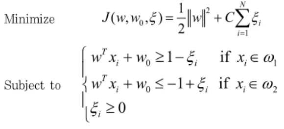
mathematical formulation. Given a set of training points, xi with respective class label yi ={1, -1}, i
= 1,2,…N, for a 2-class classification task, the SVM training algorithm computes the hyperplane (6) so as to
Minimize 0 2
1
( , , ) 1 2
N i i
J w w x w C x
=
= +
å
Subject to
0 1
0 2
1 if 1 if 0
T
i i i
T
i i i
i
w x w x
w x w x
x w
x w
x
ì + ³ - Î
ï + £ - + Î
í ï ³ î
where the margin width is equal to 2/‖w‖. The margin errors ξi are non negative; the margin errors are zeros for points outside the margin as well as in the correct side of the classifier; and they are positive for points inside the margin and on the wrong side of the classifier. C is a user-defined constant.
In many applications, SVM with a kernel function can also be used to deal with the case of non-linearly separated data sets. There are several different kernel functions used in SVMs, such as linear, polynomial, and the Gaussian radial basis functions. The selection of an appropriate kernel function is very important since the kernel defines new feature space in which the training set is linearly classified. We utilize the Gaussian radial basis kernel functions to map the input vector to a high-dimensional feature space. SVM with the Gaussian radial basis kernel function provides better performance than that with other kernel functions [18]. The Gaussian radial basic function is defined as follows:
2
2 2
( , ) ,
i j
sv sv
i j
k sv sv e s
- -
= (7)
where k(svi,svj) is the kernel function, svi and svj are the input feature vectors, and σ is a parameter set by the user to determine the width of the effective basis kernel function [18].
III. Proposed Fault Classification System
The proposed fault classification system with MLSVMs consists of two main steps: spectral envelope based cepstral coefficients (SECC) analysis, and pattern matching for classification.
The proposed fault classification system adopts hierarchical paradigm to diagnosis machine faults from the given dataset as shown in Fig. 2.
1. SECC (Spectral Envelope Cepstral Coefficients) When vibration signals are analyzed by cepstral coefficients analysis (CCA), the number of coefficients needs to be defined in advance by specifying number of filters in the filter bank and frequency intervals. In addition, frequency scales, used in CCA, are often defined by human auditory system such as melody scale, or bark scale [22].
This causes inefficiency of feature vectors in classifying faults of vibration signals. To solve this drawback, we propose another approach to automatically calculate the number of filters and define frequency intervals of the filter bank. Fig. 3 illustrates the proposed filter bank based on the
$
1
[ ] [ ],
P
k k
x n a x n k
=
=
å
- (8)1
1 1
( ) ,
( ) 1
P k k k
H z A z
a z-
=
= =
-
å
(9)spectral envelope, which consists of the following four steps.
Step 1: Eight one-second long faulty vibration signals are used to calculate linear predictive coding (LPC) coefficients {ak}m, m = 1,2,…,8 (the number of faulty symptoms), where k = 1,2,…,P and P is the order of the LPC. The spectral envelopes of vibration signals are then defined by the frequency response of an all-pole filter:
Step 2: The average spectral envelope of eight faulty vibration signals is calculated.
Step 3: The frequencies are found in which the average envelope reaches its extremes by using a gradient decent method.
Step 4: The center frequencies are given by the peak frequencies of the spectral envelope. In addition, frequency intervals are calculated by subtracting the center frequencies from the adjacent valley frequencies. With the frequency information, filter coefficients are finally defined by (3).
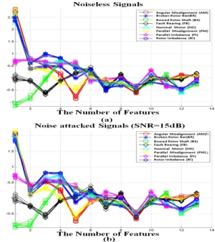
그림 3. 스펙트럴 엔벨로프 기반 필터 설계 Fig. 3. Filter design based on spectral envelope Fig. 4 shows feature vectors extracted from both
noisy and noiseless signals. The proposed feature extraction method using SECC differentiates features of each faulty vibration signal.
그림 4. SECC에 의해 추출된 특징 벡터 Fig. 4. Feature vectors extracted by SECC
2. MLSVM (Multi-Layer Support Vector Machine) In previous section, we dealt with the SVM for 2-class case. When more than two classes are present, there are several approaches that evolve around 2-class case. In this study, we utilize an one-against-all (OAA) method to consider more than two classes of feature vectors. It constructs k SVM models where k is number of classes. Each one is designed to separate one class from the rest. The ith SVM is trained with all data in the ith class with a positive label (1) and all other classes with a negative label (-1). Thus, given l training data points (x1,y1), (x2,y2),…,(xl,yl), the ith SVM solves the following problem:
Minimize 2
1
1 ( )
2
N
i i i T
j i
w C x w
=
+
å
Subject to
( ) .( ) 1 if ,
( ) .( ) 1 if ,
0 1, 2,...,
i T i i
j j
i T i i
j j
i j
w x b j i
w x b j i
j N
x x x
ì + ³ - =
ïï
+ £ - + ¹
í
ï ³ =
ïî
After training data using OAA, more than one hyperplane can have a positive value or all of them can have negative values. This problem can be solved by a multi-class SVM classifier as shown in Fig. 2. The order of SVM in the multi-layer SVM is followed by the descent order of each classifier's accuracy.
IV. Experimental Results
1. Experiment and Simulation Setup
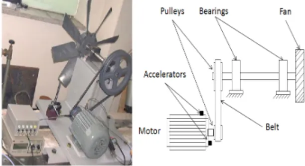
To evaluate the performance of the proposed method, we set up an experimental testbed to acquire several different faulty vibration signals as shown in Fig. 5. This setup consists of motors, pulleys, belt, shaft, and a fan with changeable blade pitch angle. Six 0.5kW, 60Hz, 4-pole induction motors were used to generate data under full load conditions. We collected one normal signal and 7 different faulty signals including angular misalignment (AM), parallel misalignment (PM), broken rotor bar (BR), bowed rotor shaft (BS), faulty bearing (FB), rotor imbalance (RI), normal (NO), and phase imbalance (PI) faults. Table 1 describes different faulty condition of the induction motor, where the acquired vibration signals were sampled at 8 kHz. In addition, we used 105 one-second long vibration signals for each faulty condition. More detailed information about this experiment is available at [5, 21].
그림 5. 유도전동기의 고장 검출을 위한 실험 시스템 Fig. 5. Experiment system for the fault detection of
induction motors
Fault Condition Fault Description angular and phase
misalignment adjusting the bearing pedestal up to 0.48o
broken rotor bar 12 EA rotor bars were broken bowed rotor shaft shaft deflection: 0.75 mm
faulty bearing a spalling on the outer race: #6203 rotor imbalance unbalance mass on the rotor: 8.4
g
phase imbalance adding resistance to one phase 표 1. 유도전동기 상태 설명
Table 1. Description of the induction motor conditions
In addition, we add additive white Gaussian noise with SNR = 10, 15, 20 dB to each normal and faulty signals. to evaluate the efficiency and robustness of the proposed method. we used 80%
feature vectors extracted from noiseless vibration signals as training data, and the rest data (feature vectors extracted from both noise-free and noise attacked signals) as testing dataset. To identify optimal sigma values set with feature vectors extracted from both noiseless and noise attacked vibration signals by using the proposed SECC analysis, we measured the classification performance with σ values in the range of 0.3 to 2.
2. System Performance with Noiseless Vibration Signals
To evaluate the performance of the proposed approach, we compare the proposed SECC with MFCC [10], STE+SVD [23] in terms of
Methods
Sigma
0.3 0.4 0.5 0.6 0.7 0.8 0.9 1 1.1 1.2 1.3 1.4 1.5 1.6 1.7 1.8 1.9 2 Fault
Type
MFCC [10]
AM 97.5 99.09 99.55 100 100 100 100 100 100 100 100 100 100 100 100 100 100 100 BR 96.14 100 100 100 100 100 100 100 100 100 100 100 100 100 100 100 100 100 BS 97.05 97.95 100 100 100 100 100 100 100 100 100 100 100 100 100 100 100 100 FB 99.32 100 100 100 100 100 100 100 100 100 100 100 100 100 100 100 100 100 NO 96.14 97.05 99.09 99.55 100 100 100 100 100 100 100 100 100 100 100 100 100 100 PM 95.91 100 100 100 100 100 100 100 100 100 100 100 100 100 100 100 100 100 PI 95.45 95.45 95.68 97.27 99.55 100 100 100 100 100 100 100 100 100 100 100 100 100 RI 97.05 97.05 97.05 97.5 97.95 98.64 100 99.77 99.77 99.77 99.77 99.77 99.77 99.77 99.77 99.77 99.77 100
STE+SVD [23]
AM 95.23 96.14 99.09 100 100 100 100 100 100 100 100 100 100 100 100 100 100 100 BR 95.45 96.14 97.95 98.64 100 100 100 100 100 100 100 100 100 100 100 100 100 100 BS 96.14 97.05 97.05 99.55 99.55 99.55 99.55 100 100 100 100 100 100 100 100 100 100 100 FB 98.64 99.55 100 100 100 100 100 100 100 100 100 100 100 100 100 100 100 100 NO 95.23 97.05 98.41 99.55 100 100 100 100 100 100 100 100 100 100 100 100 100 100 PM 96.82 99.09 100 100 100 100 100 100 100 100 100 100 100 100 100 100 100 100 PI 95 95.45 96.59 99.32 99.77 100 100 100 100 100 100 100 100 100 100 100 100 100 RI 97.05 97.05 97.5 97.95 99.32 99.77 99.77 100 100 100 100 100 100 100 100 100 100 100
SECC [proposed
]
AM 96.36 98.86 99.09 99.55 100 100 100 100 100 100 100 100 100 100 100 100 100 100 BR 97.5 99.77 100 100 100 100 100 100 100 100 100 100 100 100 100 100 100 100 BS 96.82 97.5 99.32 100 100 100 100 100 100 100 100 100 100 100 100 100 100 100 FB 100 100 100 100 100 100 100 100 100 100 100 100 100 100 100 100 100 100 NO 96.82 97.05 97.5 97.5 98.18 98.64 99.55 99.55 99.55 100 100 100 100 100 100 100 100 100 PM 96.36 100 100 100 100 100 100 100 100 100 100 100 100 100 100 100 100 100 PI 95.45 95.45 96.14 96.82 97.05 98.64 98.64 100 100 100 100 100 100 100 100 100 100 100 RI 97.05 97.5 97.95 97.95 99.09 100 100 100 100 100 100 100 100 100 100 100 100 100
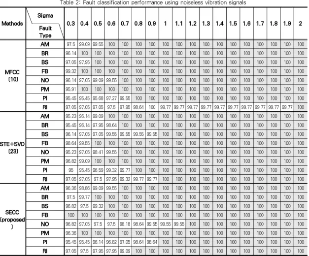
표 2. 노이즈가 없는 진동신호를 사용한 고장 분류 성능
Table 2: Fault classification performance using noiseless vibration signals classification accuracy.
Table 2 shows classification accuracy of the proposed SECC and other conventional methods with various sigma values for noiseless vibration signals.
The highest classification performance is achieved when the standard deviation (σ) of each classifier reaches to a certain value. In order to correctly classify between AM and BR, σ1 and σ2 are required more than 0.7 and 0.5, respectively. For classifying among BS, PI, and RI, the maximum performance is achieved when the values of σ3, σ7, and σ8 are not smaller than 0.6, 1, and 0.8, respectively. Furthermore, the classification accuracy is 100% when σ4 is higher than 0.3 for FB and σ6 is higher than 0.4 for PM. Finally, the
highest classification accuracy is achieved when σ5 is higher than 1.2 for nominal condition (NO). In addition to noiseless vibration signals, we also evaluate classification accuracy of the proposed method with noise attached vibration signals, which is presented in the following section.
3. Performance of Classifiers with Noise Attacked Vibration Signals
To evaluate the effectiveness of the proposed extraction method for additive white Gaussian noise signals, we train MLSVM with features extracted from original signals and measure the classification accuracy using test data including additive white
Methods Fault TypeSigma
SNR 0.3 0.4 0.5 0.6 0.7 0.8 0.9 1 1.1 1.2 1.3 1.4 1.5 1.6 1.7 1.8 1.9 2.0
MFCC [10]
AM
10 87.5 87.5 87.5 87.5 87.5 87.5 87.5 87.5 87.5 87.5 87.73 88.64 90.45 93.64 95.45 97.05 98.41 98.86 15 87.5 87.5 87.5 87.5 88.41 91.59 93.41 95.68 97.95 98.86 98.86 99.09 99.55 100 100 100 100 100 20 88.41 92.27 94.32 96.59 99.55 99.77 100 100 100 100 100 100 100 100 100 100 100 100 BR
10 87.5 87.5 87.5 87.5 87.5 87.5 87.5 87.5 87.5 87.5 87.5 87.5 87.5 87.5 87.5 87.5 87.73 87.95 15 87.5 87.5 87.5 87.5 87.5 87.73 88.64 89.77 91.14 93.64 97.05 98.64 100 100 100 100 100 100 20 87.73 90 92.27 95.68 97.5 100 100 100 100 100 100 100 100 100 100 100 100 100 BS
10 87.5 87.5 87.5 87.5 87.5 87.5 87.5 87.5 87.5 87.5 87.5 87.5 87.5 87.5 89.55 90.91 93.41 95.23 15 87.5 87.5 87.5 87.5 87.73 89.32 90.45 93.41 96.36 97.95 98.86 99.55 99.77 100 100 100 100 100 20 87.95 91.82 95.23 97.27 98.86 99.55 99.55 99.55 99.77 100 100 100 100 100 100 100 100 100 FB
10 87.5 87.5 87.5 87.5 87.73 90.68 92.73 95.45 99.32 100 100 100 100 100 100 100 100 100 15 87.5 91.14 97.05 99.55 100 100 100 100 100 100 100 100 100 100 100 100 100 100 20 97.73 99.32 99.77 100 100 100 100 100 100 100 100 100 100 100 100 100 100 100 NO
10 87.5 87.5 87.5 87.5 87.5 87.5 87.5 87.5 87.5 87.5 87.5 87.5 87.5 87.5 87.5 87.5 87.5 87.5 15 87.5 87.73 89.09 91.14 93.41 96.36 98.41 98.86 99.09 99.55 100 100 100 100 99.55 95.1 93.7 90.1 20 87.5 87.5 89.77 94.55 97.5 99.55 99.55 99.55 99.77 100 100 100 100 100 100 100 100 87.5 PM
10 87.5 87.5 87.5 87.5 87.5 87.5 87.5 87.5 87.5 87.5 87.95 88.86 90.91 91.36 93.41 95 96.14 97.27 15 87.5 87.5 87.5 87.95 88.64 90.45 92.73 96.36 97.95 98.64 99.32 100 100 100 100 100 100 100 20 87.73 89.55 96.36 97.95 99.77 100 100 100 100 100 100 100 100 100 100 100 100 100 PI
10 87.5 87.5 87.5 87.5 87.5 87.5 87.5 87.5 87.5 87.5 87.5 87.5 87.5 87.5 87.5 87.5 87.5 87.5 15 87.5 87.5 87.5 87.5 87.5 87.95 87.95 88.64 90.91 93.64 95.91 97.95 99.32 99.77 100 100 100 100 20 87.73 89.55 92.73 94.32 95.68 97.95 99.32 99.77 100 100 100 100 100 100 100 100 100 100 RI
10 87.5 87.5 87.5 87.5 87.5 87.5 87.5 87.5 87.5 87.5 87.5 87.5 87.5 87.5 87.5 87.27 87.27 86.36 15 87.5 87.5 87.5 87.5 87.5 87.27 86.82 86.14 85.45 85 85.68 87.95 90.68 92.73 92.73 93.63 93.63 93.41 20 87.5 87.5 87.95 89.55 91.82 94.55 96.14 97.27 97.95 98.41 98.41 98.41 98.41 98.41 98.18 98.18 98.18 98.18
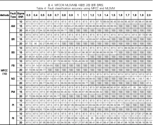
표 4. MFCC와 MLSVM을 사용한 고장 분류 정확도 Table 4: Fault classification accuracy using MFCC and MLSVM
σ1 (AM) σ2 (BR) σ3 (BS) σ4 (FB) σ5 (NO) σ6 (PM) σ7 (PI) σ8 (RI)
1.6 1.8 1.2 1.2 1.8 1.6 1.8 1.7
표 3. 가우시안 커널 함수를 가지는 MLSVM을 위한 최적의 표준 편차
Table. 3: The optimal standard deviation set for MLSVM with Gaussian kernel functions Gaussian noise. The more severely noise attacks, the
more overlapping feature vectors are generated. We observe that features extracted from the nominal (NO) and rotor imbalance (RI) conditions are overlapped. This results in decreasing classification accuracy between NO and RI.
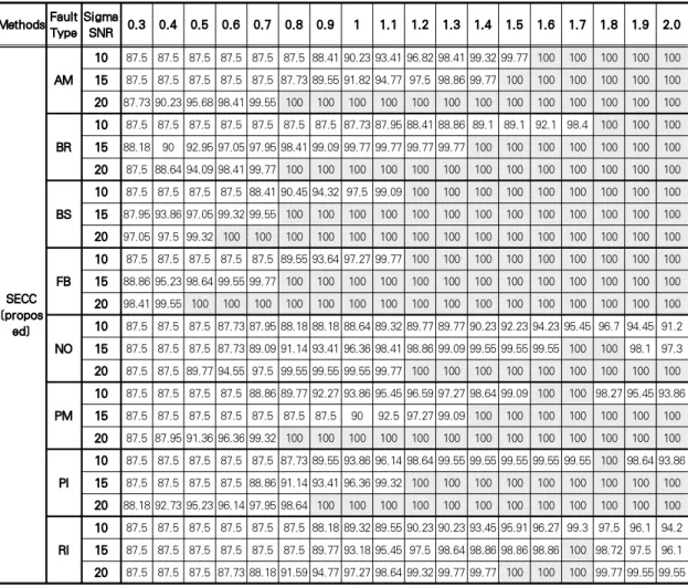
Table 3 shows selected optimal sigma values for MLSVM with Gaussian kernel functions. Tables 4, 5, and 6 show the fault classification accuracy of the conventional MFCC, STE plus SVD, and the proposed SECC, respectively. The classification accuracy of the conventional methods between NO
and RI is the lowest at SNR = 10dB, showing about 87.5%. However, the proposed SECC still provides higher classification accuracy about 96.7% and 99.3% for NO and RI, respectively, at the same SNR
= 10dB.
V. Conclusions
For early detection and classification of faults in induction motors, this paper proposed a robust feature extraction method that is cepstral coefficients based on the spectral envelope. These
MethodsFault Type
Sigma
SNR 0.3 0.4 0.5 0.6 0.7 0.8 0.9 1 1.1 1.2 1.3 1.4 1.5 1.6 1.7 1.8 1.9 2.0
STE+SV D [23]
AM
10 87.5 87.5 87.5 87.5 87.5 87.5 87.5 87.5 87.5 87.5 87.5 87.5 87.5 87.5 87.5 88.41 90 93.86 15 87.5 87.5 87.5 87.5 87.5 87.95 88.86 92.95 96.59 98.64 99.77 100 100 100 100 100 100 100 20 87.73 90 96.36 99.77 100 100 100 100 100 100 100 100 100 100 100 100 100 100 BR
10 87.5 87.5 87.5 87.5 87.5 87.5 87.5 87.5 87.5 87.5 87.5 87.5 87.5 87.5 87.5 87.5 87.5 87.5 15 87.5 87.5 87.5 87.5 87.5 87.5 87.5 87.5 87.5 87.5 87.5 87.5 87.5 87.5 87.5 87.5 87.5 87.5 20 87.5 87.5 87.5 87.5 87.5 87.5 87.5 87.5 87.5 87.5 87.5 87.5 87.5 87.5 87.73 88.18 89.32 90.45 BS
10 87.5 87.5 87.5 87.5 87.5 87.5 87.5 87.5 87.73 89.09 92.27 95.23 97.5 99.55 100 100 100 100 15 87.5 87.5 89.09 92.73 95.91 98.41 100 100 100 100 100 100 100 100 100 100 100 100 20 94.09 97.27 98.18 99.77 100 100 100 100 100 100 100 100 100 100 100 100 100 100 FB
10 87.5 87.5 87.5 87.5 88.64 93.41 98.41 100 100 100 100 100 100 100 100 100 100 100 15 88.18 96.36 100 100 100 100 100 100 100 100 100 100 100 100 100 100 100 100 20 99.32 100 100 100 100 100 100 100 100 100 100 100 100 100 100 100 100 100 NO
10 87.5 87.5 87.5 87.5 87.5 87.5 87.5 87.5 87.5 87.5 87.5 87.5 87.5 87.5 87.5 87.5 87.5 87.5 15 87.5 87.5 87.5 87.5 87.5 87.5 87.5 87.5 87.5 87.95 90 92.05 93.64 94.55 95 95.91 96.59 96.82 20 87.5 87.73 90.68 95.45 97.5 99.09 99.55 99.77 100 100 100 100 100 100 100 100 100 100 PM
10 87.5 87.5 87.5 87.5 87.5 87.5 87.5 87.5 87.5 87.5 87.5 87.5 87.5 87.5 87.5 87.5 87.73 87.95 15 87.5 87.5 87.5 87.5 87.5 87.5 87.73 89.55 93.18 96.82 99.32 100 100 100 100 100 100 100 20 87.5 87.95 94.32 99.32 100 100 100 100 100 100 100 100 100 100 100 100 100 100 PI
10 87.5 87.5 87.5 87.5 87.5 87.5 87.5 87.5 87.5 87.5 87.5 87.5 87.5 87.73 88.41 90 93.86 97.95 15 87.5 87.5 87.5 87.5 87.5 88.86 91.82 95.68 98.41 100 100 100 100 100 100 100 100 100 20 87.73 91.82 94.55 95.45 96.82 98.64 100 100 100 100 100 100 100 100 100 100 100 100 RI
10 87.5 87.5 87.5 87.5 87.5 87.5 87.5 87.5 87.5 87.5 87.5 87.5 87.5 87.5 87.5 87.5 87.5 87.5 15 87.5 87.5 87.5 87.5 87.5 87.5 87.5 87.5 87.5 87.5 87.5 87.5 87.5 87.73 88.18 89.32 90 91.36 20 87.5 87.5 87.5 87.5 88.64 89.77 93.64 95.68 96.82 97.5 98.86 99.55 99.77 100 100 100 100 100
표 5. STE+SVD와 MLSVM을 사용한 고장 분류 정확도 Table 5: Fault classification accuracy using STE+SVD and MLSVM
cepstral coefficients well reflected vibration signals with and without noise of induction motors.
Experimental results showed that the proposed method outperforms other conventional methods with the same multi-class SVMs in terms of classification accuracy.
참고문헌
[1] A. M. Da Silva, R. J. Povinelli, N.A.O.
Demerdash, “Induction Machine Broken Bar and Stator Short-Circuit Fault Diagnostics Based on Three-Phase Stator Current Envelopes,” IEEE
Transaction on Industrial Electronics, Vol. 55, pp. 1310-1318, 2008.
[2] C.-H. Hwang, Y,-M. Kim, C.-H. Kim, J.-M.
Kim, “Fault Detection and Diagnosis of Induction Motors using LPC and DTW Methods,”
Journal of the Korea Society of Computer and Information, Vol. 16, No. 3, pp. 141-147, 2011.
[3] C.-H. Hwang, M. Kang, J.-M. Kim, “A Study on Robust Feature Vector Extraction for Fault Detection and Classification of Induction Motor in Noise Circumstance,” Journal of the Korea Society of Computer and Information, Vol. 16, No. 12, pp. 187-196, 2011.
MethodsFault Type
Sigma
SNR 0.3 0.4 0.5 0.6 0.7 0.8 0.9 1 1.1 1.2 1.3 1.4 1.5 1.6 1.7 1.8 1.9 2.0
SECC [propos
ed]
AM
10 87.5 87.5 87.5 87.5 87.5 87.5 88.41 90.23 93.41 96.82 98.41 99.32 99.77 100 100 100 100 100 15 87.5 87.5 87.5 87.5 87.5 87.73 89.55 91.82 94.77 97.5 98.86 99.77 100 100 100 100 100 100 20 87.73 90.23 95.68 98.41 99.55 100 100 100 100 100 100 100 100 100 100 100 100 100 BR
10 87.5 87.5 87.5 87.5 87.5 87.5 87.5 87.73 87.95 88.41 88.86 89.1 89.1 92.1 98.4 100 100 100 15 88.18 90 92.95 97.05 97.95 98.41 99.09 99.77 99.77 99.77 99.77 100 100 100 100 100 100 100 20 87.5 88.64 94.09 98.41 99.77 100 100 100 100 100 100 100 100 100 100 100 100 100 BS
10 87.5 87.5 87.5 87.5 88.41 90.45 94.32 97.5 99.09 100 100 100 100 100 100 100 100 100 15 87.95 93.86 97.05 99.32 99.55 100 100 100 100 100 100 100 100 100 100 100 100 100 20 97.05 97.5 99.32 100 100 100 100 100 100 100 100 100 100 100 100 100 100 100 FB
10 87.5 87.5 87.5 87.5 87.5 89.55 93.64 97.27 99.77 100 100 100 100 100 100 100 100 100 15 88.86 95.23 98.64 99.55 99.77 100 100 100 100 100 100 100 100 100 100 100 100 100 20 98.41 99.55 100 100 100 100 100 100 100 100 100 100 100 100 100 100 100 100 NO
10 87.5 87.5 87.5 87.73 87.95 88.18 88.18 88.64 89.32 89.77 89.77 90.23 92.23 94.23 95.45 96.7 94.45 91.2 15 87.5 87.5 87.5 87.73 89.09 91.14 93.41 96.36 98.41 98.86 99.09 99.55 99.55 99.55 100 100 98.1 97.3 20 87.5 87.5 89.77 94.55 97.5 99.55 99.55 99.55 99.77 100 100 100 100 100 100 100 100 100 PM
10 87.5 87.5 87.5 87.5 88.86 89.77 92.27 93.86 95.45 96.59 97.27 98.64 99.09 100 100 98.27 95.45 93.86 15 87.5 87.5 87.5 87.5 87.5 87.5 87.5 90 92.5 97.27 99.09 100 100 100 100 100 100 100 20 87.5 87.95 91.36 96.36 99.32 100 100 100 100 100 100 100 100 100 100 100 100 100 PI
10 87.5 87.5 87.5 87.5 87.5 87.73 89.55 93.86 96.14 98.64 99.55 99.55 99.55 99.55 99.55 100 98.64 93.86 15 87.5 87.5 87.5 87.5 88.86 91.14 93.41 96.36 99.32 100 100 100 100 100 100 100 100 100 20 88.18 92.73 95.23 96.14 97.95 98.64 100 100 100 100 100 100 100 100 100 100 100 100 RI
10 87.5 87.5 87.5 87.5 87.5 87.5 88.18 89.32 89.55 90.23 90.23 93.45 95.91 96.27 99.3 97.5 96.1 94.2 15 87.5 87.5 87.5 87.5 87.5 87.5 89.77 93.18 95.45 97.5 98.64 98.86 98.86 98.86 100 98.72 97.5 96.1 20 87.5 87.5 87.5 87.73 88.18 91.59 94.77 97.27 98.64 99.32 99.77 99.77 100 100 100 99.77 99.55 99.55
표 6. 제안한 SECC와 MLSVM을 사용한 고장 분류 정확도
Table 6: Fault classification accuracy using the proposed SECC and MLSVM
[4] P. A. Laggan, “Vibration Monitoring,” IEE Colloquium on Understanding Your Condition Monitoring, pp. 1-11, 1999.
[5] H. Han, S. Cho, and U. Chong, “Fault Diagnosis System Using LPC Coefficients and Neural Network,” Proc. of International Forum on Strategic Technology, pp. 87-90, 2010.
[6] F. V. Nelwamonodo and T. Marwala, “Fault Detection Using Gaussian Mixture Models, Mel-Frequency Cepstral Coefficients and Kurtosis,” IEEE International Conference on Systems, Man and Cybernetics, pp. 290-295, 2006.
[7] T. Boukra and A. Lebaroud, “Classification on Induction Machine Faults,” International Multi-Conference on Systems and Devices, pp.
1-6, 2007.
[8] F. Li, G. Meng, L. Ye, and P. Chen, “Wavelet Transform-Based Higher-Order Statistics for Fault Diagnosis in Rolling Element Bearings,”
Journal of Vibration and Control, Vol. 14, pp.
1691-1709, 2008.
[9] H. Ocak, K. A. Loparo, “Estimation of the Running Speed and Bearing Defect Frequencies of an Induction Motor from Vibration Data,”
Mechanical Systems and Signal Processing, Vol.
18, pp. 515-533, 2004.
[10] F. V. Nelwamonodo, T. Marwala, and U.
Mahola, “Early Classifications of Bearing Faults Using Hidden Markov Models, Gaussian Mixture Models, Mel-Frequency Cepstral Coefficients and Fractals,” Journal of Innovative Computing, Information and Control, Vol. 2, pp. 1281-1299, 2006.
[11] M. Ge, G. C. Zhang, and Y. Yu, “Feature Extraction from Energy Distribution of Stamping Processes Using Wavelet Transform,”
Journal of Vibration and Control, Vol. 8, pp.
1323-1032, 2002.
[12] K. M. Silva, B. A. Souza, N. S. D. Brito, “Fault Detection and Classification in Transmission Lines Based on Wavelet Transform and ANN,”
IEEE Trans. on Power Delivery, Vol. 21, pp.
2058-2063, 2006.
[13] B.–S. Yang, T. Han, and W.W. Hwang, “Fault Diagnosis of Rotating Machinery based on Multi-Class Support Vector Machines,” Journal of Mechanical Science and Technology, Vol. 19, No. 3, pp. 845–858, 2005.
[14] B. –S. Yang, D.S Lim, and J.L. An, “Vibration Diagnostic System of Rotating Machinery using Artificial Neural Network and Wavelet Transform,” Proc. of 13th Intl. Congress on COMADEM, pp. 12–20, 2000.
[15] A. Widodo, B.–S. Yang, and T. Han,
“Combination of Independent Component Analysis and Support Vector Machine for Intelligent Faults Diagnosis of Induction Motors,” Expert System with Application, Vol.
32, pp. 299-312, 2007.
[16] A. Widodo, B. –S. Yang, T. Han, and D. J. Kim,
“Fault Diagnosis of Induction Motor using Independent Component Analysis and Multi-Class Support Vector Machine,”
Proceedings of the 11th Asia-Pacific Vibration Conference, pp. 144–149, 2005.
[17] S. Poyhonen, Support Vector Machine Based Classification in Condition Monitoring of
Induction Motors, Thesis Presented at Helsinki University of Technology, 2004.
[18] M. Deriche, “Bearing Fault Diagnosis Using Wavelet Analysis,” International Conference on Computers, Communication and Signal Processing with Special Track on Biomedical Engineering, pp. 197-201, 2005.
[19] N. Mehla and R. Dahiya, “An Approach of Condition Monitoring of Induction Motor Using MCSA,” International Journal of Systems Applications, Engineering and Development, Vol. 1, pp. 13-17, 2007.
[20] R. O. Duda, P. E. Hart, and D. G. Stock, Pattern Classification, Wiley, New York, 2001.
[21] T. Han, B.–S. Yang, and Z.–J. Yin,
“Feature-based Fault Diagnosis System of Induction Motors using Vibration Signal,”
Journal of Quality in Maintenance Engineering, Vol. 13, No. 2, pp. 163-175, 2007.
[22] T. H. Park, Introduction to Signal Processing:
Computer Musically Speaking, World Scientific, Singapore, 2010.
[23] M. Kang, N. Nguyen, Y. Kim, C. Kim, and J.
Kim, “Feature Vector Extraction and Classification Performance Comparison According to Various Settings of Classifiers for Fault Detection and Classification of Induction Motor,” J. of Acoustical Society of Korea, Vol.
30, No. 8, pp. 446-460, Dec. 2011.
저 자 소 개 Hung N. Nguyen
2005 : Electronics Engineering, Le Qui Dong Technical University, Vietnam, 공학사.
2011 : 울산대학교 컴퓨터정보통신공학부 석사과정 입학.
관심분야 : fault detection, signal processing Email: [email protected] 김 종 면
1995 : 명지대학교 전기공학사 2000 : University of Florida ECE
석사
2005 : Georgia Institute of Technology ECE 박사 2005 - 2007 :
삼성종합기술원 전문연구원 2007 - 현재 : 울산대학교
컴퓨터정보통신공학부 교수
관심분야 : 프로세서 설계, 임베디드 SoC, 컴퓨터구조, 병렬처리 Email: [email protected]