2003, Vol. 14, No.2 pp. 345∼354
Incremental Eigenspace Model Applied To Kernel Principal Component Analysis
ByungJoo Kim
1)Abstract
An incremental kernel principal component analysis(IKPCA) is proposed for the nonlinear feature extraction from the data. The problem of batch kernel principal component analysis(KPCA) is that the computation becomes prohibitive when the data set is large . Another problem is that, in order to update the eigenvectors with another data, the whole eigenvectors should be recomputed. IKPCA overcomes this problem by incrementally updating the eigenspace model. IKPCA is more efficient in memory requirement than a batch KPCA and can be easily improved by re-learning the data. In our experiments we show that IKPCA is comparable in performance to a batch KPCA for the classification problem on nonlinear data set.
Keywords : Kernel Principal Component Analysis, Eigenspace, Least Squares Support Vector Machine
1. Introduction
Principal Component Analysis(PCA) is a powerful technique for extracting structure from possibly high-dimensional data sets. It is easily performed by solving eigenvalue problem. PCA is an orthogonal transformation of the coordinate system in which we describe our data. The new coordinate values by which we present the data are called principal components.
In this paper, we are not focus on principal components in input space, but rather in principal components of variables, or features, which are nonlinearly related to the input variables.
An approach for nonlinear feature extraction has been taken by Tipping and
1) Professor, School of Computer & Information Engineering Youngsan University, 249 Bansong-Dong, Haeundae-gu, Busan 612-743, Korea
E-mail : [email protected]
Bishop(1998). Various global nonlinear approaches have also been developed such as auto-associative multi-layer perceptrons minimizing the reconstruction error by Diamantaras(1996) and principal curves by Kramer(1991). The disadvantage of earlier research is that they require nonlinear optimization techniques.
Recently, Scholfopf(1998) applied the kernel trick to PCA in terms of the dot product matrix instead of the covariance matrix. This makes it possible to extract non-linear features using kernel functions by solving an eigenvalue problem like PCA.
Though KPCA is capable of extracting nonlinear features, KPCA has several disadvantages. Firstly standard methods for solving eigenvalue problems need to store the entire N×N kernel matrix which can become infeasible for a large number of data N. Secondly standard PCA is usually performed in a batch mode, more specifically, requires all the training data. Thirdly in order to update the subspace of eigenvectors with another training data, we have to recompute the whole decomposition from scratch.
In this paper, we propose a incremental approach of making PCA nonlinear using empirical kernel map ΨN :Rd→RN proposed by Mika(1998), describing how an IKPCA alleviates the need for storing the kernel matrix and makes KPCA more tractable on large data sets. The empirical kernel map is briefly described in section 2. The incremental PCA outlined in section 3. The IKPCA which involves an adaption of the standard formulation of KPCA is described in section 4. In section 5 we present the results of the experiments which show the feasibility of our approach. We give the conclusion and the remark in section 6.
2. Empirical Kernel Map
The standard formulation of PCA is as the eigendecomposition of the covariance matrix of the data. Scholkopf(1998) shows that PCA can also be carried out on the dot product matrix.
Let { xN} be a data set with N examples of dimension d which is mapped into infinite dimensinal space(feature space) { Φ( xN)}. We suppose the mapped data to be centered
∑
Ni = 1xi= 0. The matrix X = [Φ( x 1),Φ( x 2),…, Φ( xN)]
represent the data in a compact way. Standard PCA is based on finding the eigenvalues and orthonormal eigenvectors of the covariance matrix in the feature space
C = 1N
∑
Ni = 1X XT. (1) We are interested in the dot product matrix of size N×N
K = 1
N XTX, (2) which is called the kernel matrix since Kij= 1
N Φ( x i)⋅Φ( xj) = 1
N k( xi,xj).
The k( xi, xj) is kernel function, which is an implicit mapping to an infinite dimensional space. KPCA is based on the fact that there is a one-to-one correspondence between the non-zero eigenvectors {vk} of C and the non-zero eigenvectors {u k} of K and that they have the same eigenvalues
λ 1, λ2, …, λ p (p ≤ min (d, N))
vk= Xuk/ λ kN (3) u k= X Tvk/ λkN (4)
where the scaling by λkN normalizes the eigenvectors. Thus, the principal eigenvectors of the covariance matrix of the mapped data lie in the span of the Φ -images of the training data.
A direct consequence of this one-to-one correspondence is that one can perform KPCA feature extraction entirely in terms of kernel functions. It requires determining the orthonormal eigenvectors u k of K and its eigenvalues λ k , and projecting a point Φ( x) onto the principal eigenvectors v k in feature space as defined by (3).
Φ( x) ⋅vk=
[ ∑i = 1N uki{Φ( x)⋅Φ( x i)}]
=[ ∑i = 1N ukik(x,xi) ]
(5)
In KPCA the data set { φ( x N)} is high dimensional and can most of the time
not even be calculated explicitly. A way around this problem is the idea of an
empirical kernel map ΨN:Rd → R N
]
(5) In KPCA the data set { φ( x N)} is high dimensional and can most of the time not even be calculated explicitly. A way around this problem is the idea of an empirical kernel map ΨN:Rd → R NΨ N(x) = [ Φ( x 1)⋅Φ( x), …, Φ( x N)⋅Φ( x)] T= [k(x1,x), …, k( xN,x)]T (6) The empirical map does not map the data into feature space but into a space of size N. This is motivated by the fact that in equation (3) the eigenvectors lie in the span of the mapped data. The empirical kernel map projects each data point onto the subspace spanned by the { φ( xN)} and enables to do all calculations in the relevant subspace of F. Since the ΨN(x N) do not form an orthonomal basis
in R N, the dot product in this space is not the ordinary dot product x⋅y =
∑
Ni = 1xiyi. But in the case of KPCA we ignore this. The idea is that we have to perform linear PCA on the ΨN(x N) from the empirical kernel map and thus diagonalize its covariance matrix. Let the N×N matrix Ψ = [ Ψ N(x1), Ψ N(x2),…, Ψ N(xN)] , then from (6) and definition of the kernel matrix Ψ = NK. This means that the covariance matrix of the empirical mapped data is
C Ψ= 1
N ΨΨT= NKKT= NK2 (7) So we actually diagonalize NK 2 instead of K as in KPCA. Mika(1998) shows that the two matrices have the same eigenvectors {u k}. The eigenvalues { λk} of K are related to the eigenvalues { k k} of NK2 by
λk= kk
N (8) and as before one can normalize the eigenvectors v k for the covariance matrix C of the data by dividing each u k by λ kN. Instead of actually diagonalize the covariance matrix C Ψ, the incremental KPCA is applied directly on the mapped data Ψ = NK. It is now relatively easy to adapt the algorithm for KPCA such that it is also correctly takes into account the centering of the mapped data in an incremental way. This means that we only need to apply the empirical map to one data point at a time and do not need to store the N×N kernel matrix.
3. Incremental Principal Component Analysis
In this section we briefly outline the method that allows for complete incremental learning using the eigenspace approach. That method uses incremental PCA algorithm and to project every input data immediately onto the subspace.
Each input data is then discarded, and its representation consists only of the corresponding principal components stored.
Let { xi} be a data set with N examples of dimension d. We compute the eigensystem by solving the singular value decomposition(SVD) of the covariance
matrix C composed as
C = 1
N
∑
n
i = 1(x i- x)( xi- x)T (9) where x = 1
N
∑
n
i = 1xi is the mean input vector.
The eigenvectors ui, i = 1…N corresponding to non-zero eigenvectors of the covariance matrix span a subspace of maximum m dimensions. We can then choose a subset of only k eigenvectors corresponding to the largest eigenvalues to be included in the model. To explain incremental PCA, we assume we have already built a set of eigenvectors U = [ u j], j = 1…k, after having used the input data xi, i = 1…N. The corresponding eigenvalues are λ = diag( Λ) where Λ is matrix of eigenvalue and x is the mean input vector. Incremental building requires to update these eigenspace to take into account a new input data x N + 1.
Here we briefly summarize the method proposed by Hall et al.(1998). First, we update the mean
x '= 1
N + 1 ( N x + x N + 1) (10) We then update the set of eigenvectors by adding a new vector and applying a rotational transformation. In order to do this, we first compute the orthogonal residual vector h = ( UaN + 1+ x) - x N + 1 and normalize it to obtain
h N + 1= h N + 1
|h N + 1|2 for | hN + 1|2> 0 and h N + 1= 0 otherwise. The new matrix of eigenvectors U ' is computed by
U '= [ U, hN + 1]R (11)
where R∈R ( k + 1 ) × ( k + 1) is a rotation matrix. R is the solution of the eigenproblem of the following form
DR = R Λ' (12) We compose D∈R ( k + 1 ) × ( k + 1) as
D = N
N + 1
[
0Λ 0T 0]
+ N( N + 1) 2
[
aaγa TT γaγ2]
(13)where γ = hTN + 1(xN + 1- x) and a = UT(x N + 1- x). There are other ways to construct matrix D. However, only the method proposed by Hall et al.(1998) allows for the updating of mean.
4. Incremental Kernel Principal Component Analysis
Although incremental PCA builds the subspace of eigenvectors incrementally, it is limited to linear data. For the case of nonlinear data set, applying feature mapping function method to incremental PCA may be the solution. This is performed by kernel-trick as described in section 2 ,which is an implicit mapping to an infinite dimensional space.
K( x, y) =Φ( x) ∙Φ( y) (14)
Where K is a given kernel function in input space. When K is semi positive definite, the existence of Φ is proved by Vapnik(1998). But, most of the case the mapping Φ cannot be obtained explicitly, so the vector in the feature space is not observable and only the inner product between vectors can be observed via kernel function. So in this paper we take empirical kernel map described in Section 2. Tsuda(1999) shows that support vector machine with empirical kernel map is identical with the conventional kernel map.
5. Experiment
First we shall take a look at simple toy data which will show the validation of IKPCA. It is done by comparing the eigenvector of IKPCA with batch KPCA.
Next we will evaluate the usefulness of the nonlinear feature extraction by IKPCA, as a preprocessing step for classification. For this purpose, extracted features by IKPCA will be used for training simple linear classifier. Among many linear classifier, we take linear least squares support vector machine(LS-SVM) proposed by Suyken(1999). The reason why we use LS-SVM in this paper is that LS-SVM method is computationally attractive and easier to extend than standard support vector machine. In order to evaluate the IKPCA feature extraction capability, experiments were carried out two class and multiclass data classification problem.
5.1 IKPCA versus Batch KPCA
To evaluate the performance of IKPCA and batch KPCA we take nonlinear data used by Scholkoff(1998). Training data set is generated by
y = x2+ 0.2ε : ε∼N( 0, 1), x = [ - 1, 1] (15) In Figure 1 upper part is batch KPCA and lower is IKPCA. From left to right the first 3 eigenvalues are shown in decreasing order. Contour lines indicate constant principal component value. We can see that there is a close similarity between batch KPCA and IKPCA in contour graph and eigenvalues .
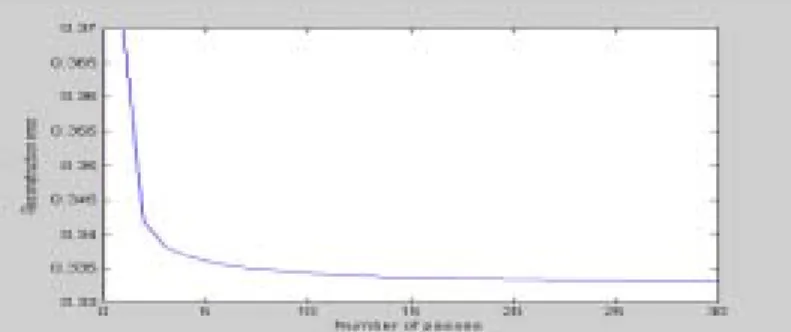
Another factors of performance evaluation are reconstruction error and eigenvector's cosine value similarity between IKPCA and batch way KPCA.
Reconstruction error is defined as the squared distance between the Ψ image of x N and its reconstruction when projected onto the first l principal components.
δ = | Ψ( x N)- P lΨ( xN)|2. (16) Figure 2 shows the reconstruction error by re-learning in IKPCA. SSE(Sum of Square Error) and MSE(Mean Square Error) value of reconstruction error is 0.36975 and 0.0090. This means the performance of IKPCA is similar to batch KPCA.
Finally, to check the similarity of eigenvectors of both methods we compute the cosine values between each eigenvector of KPCA and the corresponding of IKPCA. B and I are the matrices of eigenvectors of batch KPCA and IKPCA, respectively.
Fig. 1. Two-dimensional toy examples, with data was generated in Eq.(15). Upper part is batch KPCA and lower is IKPCA
Fig. 2. Reconstruction error change by re-learning in IKPCA
.
−
−
−
−
=
13795 . 0 85384 . 0 11171 . 0
5259 . 0 11002 . 0 82981 . 0
19613 . 0 49981 . 0 094315 . 0
81604 . 0 095116 . 0 53856 . 0 B
−
−
−
−
=
13649 . 0 85384 . 0 11171 . 0
52635 . 0 11002 . 0 82981 . 0
19364 . 0 49981 . 0 094314 . 0
8166 . 0 095114 . 0 53856 . 0 I
Table 1 shows the cos θ and θ values ,which shows the similarity of eigenvectors of both methods.
Table1. Eigenvector's cos θ and θ value obtained by IKPCA and batch KPCA
Eigenvector ∣ cos θ ∣ θ
1 1 0
2 1 0
3 1 0
The results of simple toy problem indicate that the proposed method is comparable to the batch way KPCA.
5.2 Two Class Classification
In two class classification problem, we use two data set. Classical benchmarking data and real world data.
5.2.1 Two-Spiral Data
Two-spiral classification problem is known to be hard for multilayer perceptrons. Here we test a spiral problem for which two classes have been defined and each class has 60 training data points. A RBF kernel has been taken
with σ 2= 0.1. Correct classification ratio of linear LS-SVM is 100%. By this result, we can see that IKPCA extracts nonlinear features well.
5.2.2 Real World Data
To test the performance of IKPCA for real world data, we use Cleveland heart disease data obtained from the UCI Machine Learning Repository. Data set has 303 patterns and each pattern has 13 attributes.The two classes are highly overlapped. Goal is to distinguish between presence and absence of heart disease in a patient. Like two-spiral data classification problem, same procedure is applied.
A RBF kernel has been taken with σ2= 0.1. Correct classification ratio of linear LS-SVM is 100%. By this result, we can see that IKPCA extracts nonlinear features well on real world data.
5.3 Multi Class Data
Earlier experiments was carried to classify two class problem. Here we extend experiment to multiclass classification problem. Training data is wine data obtained from the UCI Machine Learning Repository. Wine data are the results of a chemical analysis of wines grown in the same region in Italy but derived from three different cultivates. The analysis determined the quantities of 13 constituents found in each of the three types of wines. Detailed attributes are available from web site( http://www.ics.uci.edu/~mlearn/MLSummary.html).
Number of instances per class is 59 for class 1, 71 for class 2, and 48 for class 3. In this case we use classifier as multiclass LS-SVM proposed by Suyken(1999).
The three classes have been encoded by taking m = 2. A RBF kernel has been taken with σ21= σ22= 0.1 and γ = 1. Correct classification ratio of linear milticlass LS-SVM is 100%.
6. Conclusion and Remarks
This paper was devoted to the exposition of a new technique on extracting nonlinear features from incremental data. To develop this technique, we made use of empirical kernel mapping with incremental learning by eigenspace approach.
Proposed IKPCA has following advantages.
Firstly, IKPCA has similar feature extracting performance for incremental and nonlinear data comparable to batch KPCA. Secondly, IKPCA is more efficient in memory requirement than batch KPCA. In batch KPCA the N×N kernel matrix has to be stored, while for IKPCA requirements are O( ( k + 1)2). Here
k( 1≤k≤N) is the number of eigenvectors stored in each eigenspace updating step, which usually takes a number much smaller than N. Thirdly, IKPCA allows for complete incremental learning using the eigenspace approach, whereas batch KPCA recomputes whole decomposition for update the subspace of eigenvectors with another data. Fourthly, IKPCA can easily be improved by re-learning the data. Fifthly IKPCAdo not require nonlinear optimization techniques. Lastly, experimental results show that extracted features from IKPCA lead to good performance when used as preprocess data for a linear classifier.
Future works is combining IKPCA with excellent classifier so make the system do well in classification task.
References
1. Diamantaras, K.I., & Kung, S.Y. (1996). Principal Component Neural Networks: Theory and Applications. New York John Wiley & Sons, Inc.
2. Hall, P., Marshall, D., & Martin, R. (1998). Incremental eigenalysis for classification. In British Machine Vision Conference, (Vol.1). pp. 286-295.
3. Hall, P., Marshall, D., & Martin, R. (2000). Merging and splitting eigenspace models. PAMI, 22(9): pp1042-1048, .
4. Kramer, M.A. (1991). Nonlinear principal component analysis using autoassociative neural networks. AICHE Journal 37(2), 233-243.
5. Mika, S. (1998). Kernalgorithmen zur nichtlinearen Signal verarbeitung in Merkmalsraumen. Master's thesis, Technische Universitat Berlin November. http://www.first.gmd.de/~mika/diplom.ps.gz
6. Scholkopf, B., Smola, A. & Muller, K.R. (1998). Nonlinear component analysis as a kernel eigenvalue problem. Neural Computation 10(5), 1299-1319 .
7. Scholkopf, B., Mika, S., Burges, C., Knirsch, P., Muller, K.R, & Smola, A. (1999). Input Space versus Feature Space in Kernel- based Methods.
IEEE Transactions on Neural Networks, vol. 10, 1000- 1017.
8. Tipping, M.E., & Bishop, C.M. (1998). Mixtures of probabilistic principal component analysers. Neural Computation 11(2), 443-482.
9. Tsuda, K. (1999). Support vector classifier based on asymmetric kernel function. Proc. ESANN .
10. Suyken, J.A.K. and Vandewalle(1999). Least squares support vector machine classifiers. Neural Processing Letters, vol.9, pp293-300 . 11. Vapnik V. N. (1998). Statistical learning theory. John Wiley & Sons,
New York, .
[ received date : Feb. 2003, accepted date : Apr. 2003 ]