A Study of Frequency Mixing Approaches for Eddy Current Testing of Steam Generator Tubes
Hee Jun Jung*, Sung-Jin Song*✝, Chang-Hwan Kim* and Dea Kwang Kim*
Abstract The multifrequency eddy current testing(ECT) have been proposed various frequency mixing algorithms.
In this study, we compare these approaches to frequency mixing of ECT signals from steam generator tubes;
time-domain optimization, discrete cosine transform-domain optimization. Specifically, in this study, two different frequency mixing algorithms, a time-domain optimization method and a discrete cosine transform(DCT) optimization method, are investigated using the experimental signals captured from the ASME standard tube. The DCT domain optimization method is computationally fast but produces larger amount of residue.
Keywords: Multifrequency Mixing, ECT, DCT, Optimization, Steam Generator Tube
Received: November 13, 2009. Revised: December 11, 2009. Accepted: December 14, 2009. *School of Mechanical Engineering, Sungkyunkwan University, 300, Chunchun-dong Jangan-gu, Suwon 440-746, Korea, ✝Corresponding Author: [email protected]
Journal of the Korean Society for Nondestructive Testing Vol. 29, No. 6 (2009. 12)
1. Introduction
Steam generator tubes are held at regular intervals by tube support plates(TSP) and are surrounded by a mixture of water and steam.
Over a period of time the support plates react with the mixture which results in an accumulation of oxides in gap regions between a tube and plates. Eddy current testing(ECT) of nondestructive evaluation(NDE) plays an important role in assessing the structural integrity of steam generator tubes in nuclear power plants(Arunchalam et al., 2002).
ECT by its nature is sensitive to any change in the electrical or magnetic properties of the test part. Steam generator tubes include not only defects, but also support structures, electrically conductive deposits, permeability variations, dents and bulges, roll expansions and other phenomena.
Indications from all these unwanted effects combine with indications from defects so that both flaw detection and sizing become difficult.
The multifrequency ECT method is a data analysis method which analyzes the signal in the impedance plane using different frequencies. In general, lower frequencies give deeper penetration but would yield reduced sensitivity and poor discrimination between surface and subsurface defects. Higher frequencies would make subsurface defects undetectable. According to the frequency dependence of the impedance change response, we can have different sensitivities of a defect signal at different frequencies. With the multifrequency ECT method, we can analyze these signals simultaneously and use characteristics of the defects and other unwanted parameters on different frequencies to identify the flaw indications.
For the multifrequency ECT method, data from individual frequencies are combined by a vector addition process. This combination of data is referred to as mixing and is mathematically equivalent to simultaneous solution of multiple equations. This mixing process permits
elimination of unwanted test parameters while those of interest are retained. In steam generator inspection the desired information on tubing flaws can be masked by dents, support plates, probe wobbles, and inside-diameter variations such as mandrel chatter or pilfering.
With the multifrequency ECT method, we can suppress those unwanted test variables. This is especially important for flaws near tube support plate regions: an accurate estimation of the flaw depth is only possible after the support plate signal is removed.
This study presents a technique for processing multifrequency data to eliminate unwanted signals. Examples of unwanted signals include support plates, dents and magnetite deposits on the outside of tubes. These signals sometimes mask harmful defect signals.
Multifrequency processing techniques can be employed to suppress the unwanted signals without degrading the quality of defect signals.
One important processing procedure in multifrequency testing is the mixing of the signals from different frequency channels. It can be used to separate a flaw signal from a support plate signal for flaws near support plate structures. Frequency mixing can be implemented in hardware by using multipliers and adders. It can also be implemented in software by using a least squares(LS) algorithm or the other similar algorithms. Frequency mixing provides an advantage which is not possible in single frequency eddy current testing: the mixed channel can be tuned to be sensitive to certain types of defects and to eliminate signals from structures which are of no interest to the inspector(Chuang, 1997).
2. Frequency Mixing
The concept of frequency mixing is quite simple but the results of most currently available mixing algorithms are far from ideal as shown in Fig. 1. At this time, there is still no industrial
standard mixing algorithm. Most companies use their own proprietary mixing algorithms. The mixing algorithm is very important because a large number of flaws occur near or within the tube support plate area and their signals are distorted by the TSPs(Lord, 1985).
Frequency mixing is a technique used to suppress unwanted signals in multiple frequency measurement data. It is based on the assumption that the signals from different channels can be represented by different linear combinations of several test variables.
The first order of business relative to the development a viable multifrequency eddy current inspection procedure is the selection of appropriate system operating frequencies. A basic frequency is first chosen, then secondary frequencies to meet the test requirements for optimum detection and characterization of all defect conditions, including under extraneous signals which necessitates a mixing process. The basic frequency is that which might normally be used when conducting a single frequency eddy current examination. The two major parameters to be considered are the depth of penetration of eddy current through the tube wall, which is related to the OD to ID sensitivity ratio and the phase angle between shallow ID and OD defect signals. The selection of a secondary frequency for mixing purpose must satisfy several criterions. The first parameter to consider is the ratio of amplitudes between a standard defect and the unwanted signal. This ratio must be much smaller at the second frequency(Pintiere, 1980). Recently, the selection procedure of basic and auxiliary frequency is according to EPRI guidelines.
Through rotation and scaling and subtraction of signals from different channels, we may obtain the wanted test variable while suppressing unwanted test variables. In its hardware implementation, the optimal rotation and scaling factors are reached by visual inspection of the residue signal. In the software implementation, it
( ) ( )
⎥⎥⎥
⎦
⎤
⎢⎢
⎢
⎣
⎡
+
−
−
=
θ θ
θ θ
θ θ
θ θ
cos sin
cos sin sin
cos sin cos
y x
y y y
y x
x x x
T T
S S S T
T S
S S A
(3)
aA
b C
C
d
= −
(4)F1 F2
M1
Basic Frequency Auxiliary Frequency
Support Plate Suppressed
-200-150-100-50 0 50 100 150 200
-500 -400 -300 -200 -100 0 100 200 300 400 500
-800-600-400-200 0 200400 600800
-2500 -2000 -1500 -1000 -500 0 500 1000 1500 2000 2500
-200-150-100-50 0 50 100 150 200
-500 -400 -300 -200 -100 0 100 200 300 400 500
F1 F2
M1
Basic Frequency Auxiliary Frequency
Support Plate Suppressed
-200-150-100-50 0 50 100 150 200
-500 -400 -300 -200 -100 0 100 200 300 400 500
-800-600-400-200 0 200400 600800
-2500 -2000 -1500 -1000 -500 0 500 1000 1500 2000 2500
-200-150-100-50 0 50 100 150 200
-500 -400 -300 -200 -100 0 100 200 300 400 500
Fig. 1 A schematic representation of the mixing algorithm
is usually assumed that the unwanted signal is much larger than the wanted signal, and thus the aim is to minimize the residue signal in the least-squares sense.
Suppose the signal at the higher frequency is the linear combination of the flaw signal and the unwanted signal, while the signal at the lower frequency is the unwanted signal only. The unwanted signal in the higher frequency is represented as scaled and rotated version of the signals in the lower frequency.
A theory on the mixing of multifrequency eddy current data in both the time domain and the frequency domain was presented(Stolte et al., 1988). A fundamental assumption made in this theory is that eddy current signals at two frequencies are an affine transformation of each other(Avanindra, 1997). For the tube support plate regions, the steps for suppressing the contribution due to the tube support plates are described as follows,
1. Let
and
be the support plate signals at the auxiliary frequency signal and the basic frequency signal.2. Let
where an affine transformation
is a function of
: scaling in x direction
: scaling in y direction
: translation in x direction
: translation in y direction
: rotation about the originThe sequence
′
is obtained using the transformation[ ] [
x y' =
xy1 ]
A (1)(
x y x y)
a a
b S S T T S S
S
=
'=
A, , θ , ,
(2)where an affine transform matrix
is given by3. Let
and
be the composite (support plate and defect) signals at the auxiliary frequency signal and the basic frequency signal. Then the defect signal is given by eqn.(4)The most important step of mixing is to find the transformation parameters using the measured signals of the tube support plate (or other signals to be suppressed) at the two frequencies. The transformation can be implemented in both time domain and the frequency domain.
3. Discrete Cosine Transform
The discrete cosine transform(DCT) of a data sequence,
…
is defined as eqns. (5) and (6)( ) ∑
−( )
=
=
10
0 1
nm
x X m
G n (5)
( ) ( ) ( )
( )
1 0
2 1
2 cos ,
2 1, 2, , 1
n x
m
m k
G k X m
n n
k n
π
−
=
= +
= −
∑
L
(6)
where
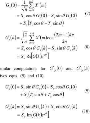
is the kth DCT coefficient and this coefficient gives eqns. (7) and (8)( ) ( )
( ) ( )
( θ θ )
θ θ
sin cos
0 sin 0
cos
0 1
10 ' '
y x
x
y x
x x
n m x
T T
S
G S
G S
m n X
G
− +
−
=
= ∑
−= (7)
( ) ( ) ( )
( ) ( )
[ θ ( ) θ] θ
π
j x
y x x x
n m x
e k G S
k G S
k G S
n k m m
n X k G
Re
sin cos
2 1 cos 2 2
10 ' '
=
−
=
= ∑
−+
=
(8)
Similar computations for
′
and′
gives eqns. (9) and (10)
( ) ( ) ( )
( θ θ )
θ θ
cos sin
0 cos 0
sin
'
0
y x
y
y y
x y y
T T
S
G S
G S G
+ +
+
=
(9)( ) ( ) ( )
[ θ ( ) jθ] θ
y
y y
x y y
e k G S
k G S
k G S
k G
Im
cos
'
sin
=
+
=
(10)The equations clearly show the relation between the DCT coefficients of sequences
and′
. Given the DCT coefficients of sequences
and
, it is possible to use the eqn. (2) to calculate the values of the translation parameters. The affine transform parameters
can be calculated as follows.( ) ( ) [ ( ) ] [ ( )
θ]
θ j j
x x k
k Gk e
e k G k
G k R G
2 1 2
' 1 '
Re Re
2
1
= =
(11)Expanding the eqn. (11) and rearranging the terms gives eqn. (12);
( ) ( )
( )
22( )
112 1
2
tan
1k G k G R
k G k G R
y y
k k
x x
k k
−
= −
θ
(12)After
is estimated,
and
can be calculated using the eqns. (8) and (10).
and
are calculated from eqns. (7) and (9) relating the zeroth DCT coefficients of the two signals. All other terms in the equations are known, consequently the two equations can be solved simultaneously for
and
.The DCT algorithm for finding the optimal affine transform parameters is implemented using the related equations. The DCT coefficients are calculated for the basic and the auxiliary frequency signals. These coefficients can be evaluated efficiently using fast algorithms.
Another noteworthy aspect of this procedure is that only a few DCT coefficients need to be calculated. This reduces the computational burden even further once the DCT coefficients are calculated, the optimal transform parameters can be estimated using the related equations.
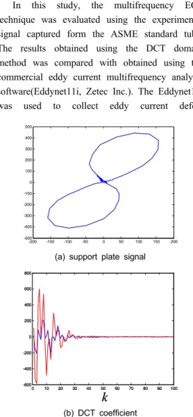
Consequently, we found the optimum number of coefficients as can be seen in Fig. 2. The red line is resistance component and the blue line is reactance component.
The parameters can be estimated using any arbitrary value of
. However, it has been observed that not all coefficients provide identical estimates of the parameters. The closed form relations between the DCT coefficients of the basic and auxiliary frequency signals suggests that invariant feature vectors can be found which would be insensitive to translation, rotation and scaling of the original signal. These invariant features are dependent only on the shape of the impedance plane trajectory. So, we have to solve nonlinear least squares problem. In this study, the results are the same as those obtained using the conjugate gradient method with time-domain optimization method.Especially, we adopted the Levenberg-Marquardt gradient decent method in the function of MATLAB. The error function E is the function of
. To minimize the E is defined as eqn. (13)' 2
' 2
([ ( ) ( )]
[ ( ) ( )] )
x x
y y
Min E G k G k G k G k
= − +
−
∑
(13)Fig. 3 shows the results obtained using the DCT domain optimization algorithm for calculating the optimal affine transform parameters for the experimental data.
-200 -150 -100 -50 0 50 100 150 200 -500
-400 -300 -200 -100 0 100 200 300 400 500
(a) support plate signal
0 10 20 30 40 50 60 70 80 90 100
-600 -400 -200 0 200 400 600 800
0 10 20 30 40 50
k
60 70 80 90 100-600 -400 -200 0 200 400 600 800
k
(b) DCT coefficient
Fig. 2 DCT coefficients for a support plate signal
-800 -600 -400 -200 0 200 400 600 800
-2500 -2000 -1500 -1000 -500 0 500 1000 1500 2000 2500
(a)
-800 -600 -400 -200 0 200 400 600 800
-2500 -2000 -1500 -1000 -500 0 500 1000 1500 2000 2500
(b)
-200 -150 -100 -50 0 50 100 150 200
-500 -400 -300 -200 -100 0 100 200 300 400 500
(c)
-500 0 500
-500 -400 -300 -200 -100 0 100 200 300 400 500
(d)
Fig. 3 Mixing results using DCT domain optimization method for (a) support plate (400 kHz) (b) support plate (100 kHz) (c) transformed support plate signal (d) mixed support plate signal
Fig. 3 presents the step by step method for support plate suppression. First, the support ring was placed on a defect free region of the tube.
The tube was scanned and pure support plate signatures were obtained. These are displayed in Fig. 3(a) and (b). The mixing parameters were calculated form these signals and stored. The tube was scanned again, to locate and characterize flaws in the tube. Fig. 3(c) shows the auxiliary support signal (dotted lines) translated to map the basic frequency support signal which is also displayed. The result of subtraction is shown in Fig. 3(d). As can be see, the residual signal after subtraction is small.
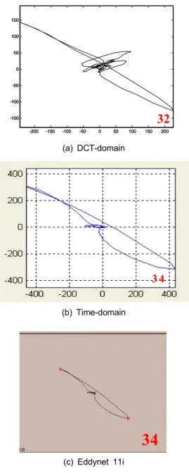
In this study, the multifrequency ECT technique was evaluated using the experimental signal captured form the ASME standard tube.
The results obtained using the DCT domain method was compared with obtained using the commercial eddy current multifrequency analysis software(Eddynet11i, Zetec Inc.). The Eddynet11i was used to collect eddy current defect
-200 -150 -100 -50 0 50 100 150 200 -150
-100 -50 0 50 100 150
32
-200 -150 -100 -50 0 50 100 150 200
-150 -100 -50 0 50 100 150
32
(a) DCT-domain
3 4 3 4
(b) Time-domain
34 34
(c) Eddynet 11i
Fig. 4 Comparison of mixing algorithms and commercial software result for a TWH defect signatures at multiple excitation frequencies in the presence of a support plate.
Fig. 4 shows the result of subtraction of the translated composite signal from the basic composite signal when the support ring is placed above the through wall hole(TWH) defect. The support plate signal is completely suppressed.
Fig. 4(c) shows the results obtained from the commercial software. The algorithm used by the
commercial software for calculating the transformation parameters is not known.
However, a comparison as shown in Fig. 4 shows that similar results can be obtained from the DCT-domain optimization method, Time-domain optimization method and the Eddynet11i software. The DCT-domain optimization method is faster than time-domain optimization method, but, as we have seen the DCT-domain optimization method remain a larger amount of residue.
4. Summary
The frequency mixing approach that is applied in this study uses composite signals for calculating the transformation parameters. The parameters are used to translate the auxiliary frequency signal to nullify the effect of the support plate. An outcome of the study is that the discrete cosine transform based features that are insensitive to rotation, scaling and translation of the original signal can be obtained. The results obtained using the time domain optimization method and the DCT domain optimization methods are similar to those obtained using the Eddynet11i when the support plate signal is used for mixing or when the composite signals are directly mixed. It should be concluded that the DCT domain optimization method is computationally fast but produces larger amount of residue.
Acknowledgments
This work was supported by the Korea Science and Engineering Foundation(KOSEF) grant funded by the Korea government (MEST) (No. 2009-0067250)
References
Arunchalam, K., Ramuhalli, P., Udpa, L. and Udpa, S (2002) Nonlinear Mixing Algorithms for
Suppression of TSP Signals in Bobbin Coil Eddy Current Data, Review of Progress in Quantitative Nondestructive Evaluation., Vol. 21, pp. 631-638
Chuang, S. (1997) Eddy Current Automatic Flaw Detection System for Heat Exchange Tubes in Steam Generators, Ph.D. Thesis, Iowa State University
Lord, W. (1985) Electromagnetic Methods of Nondestructive Testing, Gordon and Breach Science Publishers, USA
Pintiere, L. (1980) An Analysis of Multifrequency Eddy Current Mixing Parameters in Tubing Inspection, Nondestructive Evaluation in the Nuclear Industry, USA
Stolte, J., Udpa, L. and Load, W. (1988) Multifrequency Eddy Current Testing of Steam Generator Tubes Using Optimal Affine Transform, Review of Progress in Quantitative Nondestructive Evaluation, Vol. 7A, pp. 821-830 Avanindra (1997) Multifrequency Eddy Current Signal Analysis, M.S. Thesis, Iowa Stats University