C OMPUTATION OF T URBULENT N ATURAL C ONVECTION IN A R ECTANGULAR C AVITY WITH THE F INITE- V OLUME
BASED L ATTICE B OLTZMANN M ETHOD
Seok-Ki Choi *1 and Seong-O Kim 2
유한체적법을 기초한 레티스 볼쯔만 방법을 사용하여 직사각형 공동에서의 난류 자연대류 해석
최 석 기,
*1
김 성 오2
A numerical study of a turbulent natural convection in an enclosure with the lattice Boltzmann method (LBM) is presented. The primary emphasis of the present study is placed on investigation of accuracy and numerical stability of the LBM for the turbulent natural convection flow. A HYBRID method in which the thermal equation is solved by the conventional Reynolds averaged Navier-Stokes equation method while the conservation of mass and momentum equations are resolved by the LBM is employed in the present study.
The elliptic-relaxation model is employed for the turbulence model and the turbulent heat fluxes are treated by the algebraic flux model. All the governing equations are discretized on a cell-centered, non-uniform grid using the finite-volume method. The convection terms are treated by a second-order central-difference scheme with the deferred correction way to ensure accuracy and stability of solutions. The present LBM is applied to the prediction of a turbulent natural convection in a rectangular cavity and the computed results are compared with the experimental data commonly used for the validation of turbulence models and those by the conventional finite-volume method. It is shown that the LBM with the present HYBRID thermal model predicts the mean velocity components and turbulent quantities which are as good as those by the conventional finite-volume method. It is also found that the accuracy and stability of the solution is significantly affected by the treatment of the convection term, especially near the wall.
Key Words : Lattice Boltzmann method, Finite volume method, Turbulent flow, Natural convection,
Turbulence modeling, HYBRID LBM접수일: 2011년 10월 15일, 수정일: 2011년 10월 28일, 게재확정일: 2011년 10월 30일.
1 정회원, 한국원자력연구원 2 정회원, 한국원자력연구원
* Corresponding author, E-mail: [email protected]
1. I NTRODUCTION
Accurate prediction of natural convection flows is very important for investigating various engineering applications such as cooling of electronic packages, solar collector, building ventilation and passive heat removal system of a
liquid metal nuclear reactor. The Rayleigh number of most practical flows for engineering applications is at least larger than
and the direct numerical simulation or large eddy simulation methods can not applied to these practical engineering flows. Most works in the literature employ the Reynolds-Averaged Navier-Stokes (RANS) equation approach. In the present study we present numerical results of turbulent natural convection flow computed by the lattice Boltzmann method(LBM) together with the RANS equation method.The LBM has received a great deal of attention during last two decades mainly due to its algorithm simplicity.
The conventional Lagrangian type LBM comprises streaming and collision steps and these steps are computed algebraically. Thus, the numerical solution of partial differential equation is not needed. It is also relatively easy to implement the solution procedure in a massively parallel computer. Therefore, the LBM can take full advantage of parallel computation. In the Eulerian type LBM such as the finite-volume or finite-element based methods, the linear hyperbolic equations for the particle distribution functions are solved. This facilitates the time marching solution procedure without inner iteration. Due to these advantages many authors employed the LBM for numerical solutions of fluid flow and heat transfer problems[1].
One of the limitations of the conventional LBM has been the lack of an accurate and stable thermal model for heat transfer problems. There exist four thermal models in conjunction with the LBM: the multispeed approach[2], the passive scalar approach[3], the double-population approach[4] and the HYBRID method. The merits and demerits of above four thermal models are explained well in Peng et al.[5]. At present the multi-speed approach and the passive scalar approach are not used due to the numerical instability problems. In the HYBRID method the Navier-Stokes equation method is employed only for the solution of the energy equation while the conservation of mass and momentum is resolved by the LBM. By this way the full advantages of the LBM and the Navier-Stokes equation method are taken. Only one energy equation needs to be solved. Recently Choi and Kim[6]
compared the relative performance between the double-population approach[4] and the HYBRID method for the laminar natural convection in a square cavity.
The computed results showed that the finite-volume based HYBRID and double-population LBM are as accurate as the Navier-Stokes equation method. The relative performance between the HYBRID and double-population LBM shows that the HYBRID method shows better convergence and stability than the double-population method. When the double-population method is used, the introduction of additional nine internal energy (or temperature) distribution functions in a two-dimensional situation (D2Q9) adds to the complexity of the algorithm.
The HYBRID method is simple to implement and is an economic way of implementing the thermal equation with the LBM. Following these observations, the HYBRID method is used for the numerical solution of turbulent natural convection in the present study.
Computation of turbulent flow is one of the most
challenging subjects of CFD. Most practical engineering problems occur at high Reynolds or Rayleigh number and it is still too time consuming to perform a direct numerical simulation or a large eddy simulation for such flows using the present computers. Thus, introduction of RANS (Reynolds-Averaged Navier-Stokes) equation method in conjunction with the LBM is needed for numerical solution of practical engineering problems and such works are reported in the literature, such as the works by Teixeira[7] and Choi and Lin[8]. Within the present author’s knowledge only one work by Zheng et al.[9] is reported in the literature which computed the turbulent natural convection by the RANS equation method with the LBM. The authors used the RNG
model with the wall function method. In the present study the elliptic-relaxation turbulence model by Medic and Durbin[10] is used to compute the turbulent natural convection in a rectangular cavity. Medic and Durbin[10]developed an elliptic-relaxation model in which two more partial differential equations than the conventional
model are solved to determine the velocity scale in the expression of turbulence eddy viscosity. Choi et al.[11]applied this model to the computation of natural convection in a rectangular cavity and showed that this model outperforms the conventional
models.The other difficulty in predicting the turbulent natural convection is the treatment of the turbulent heat fluxes.
If one does not use the differential heat flux model, a proper way of treating the turbulent heat fluxes should be sought. In the earlier stage of works the present authors used a simple gradient diffusion hypothesis (SGDH) in treating the turbulent heat fluxes. However, it does not work well for the natural convection flows. Ince and Launder[12] proposed a generalized gradient diffusion hypothesis(GGDH) to overcome this deficiency of the SGDH assumption. The GGDH works very well for the shear dominant flows, however it produces unstable and inaccurate solutions for the strongly stratified natural convection flows. To remedy this deficiency, Kenjeres and Hanjalic[13] developed an algebraic flux model (AFM). The main difference between the AFM and the GGDH is the inclusion of the temperature variance term in the algebraic expression of the turbulent heat fluxes.
This inclusion of temperature variance term stabilizes the overall solution process and results in stable and accurate solution. However, the AFM requires one more numerical solution of a partial differential equation for the temperature variance than the GGDH.
The main objective of the present study is to
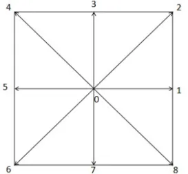
Fig. 1 A schematic diagram of velocity directions of D2Q9 model
investigate the performance of the HYBRID LBM for turbulent natural convection in an enclosure using the RANS equation method. A brief introduction is given above and the mathematical formulations of the LBM and the details of turbulence model will be given in the following section. This is followed by the results and discussion, and a brief conclusion is drawn.
2. M ATHEMATICAL FORMULATION
2.1 G OVERNING EQUATIONS
The discrete Boltzmann equations with Bhatnagar-Gross-Krook collision operator can be written as follows;
∙ ∇
(1)for
where
is the particle distribution function,
is the discrete microscopic velocity vector,
is the relaxation time and
is the equilibrium distribution function obtained by Taylor expansion of the Maxwell-Boltzmann distribution function. It is noted that the repeated Greek subscript in above equation does not imply summation.
In the most commonly used D2Q9 lattice, shown in Fig.
1, the discrete particle velocity vector
is expressed as,
cos
sin
cos
sin
(2)
The equilibrium distribution function takes the form
∙
∙
∙
(3) and the weighting factor
is given as follows;
(4) The macroscopic density
and the velocity vector
are related to the distribution function by
(5)The pressure can be calculated from
with the speed of sound
and the kinematic viscosity of fluid is
. The forcing term in Eq.(1) is given by He et al.[4] as follows; ∙
(6)
2.2 B OUNDARY CONDITIONS
The treatment of boundary conditions in the LBM is one of the major concerns not fully resolved until now.
Several different treatments of wall boundary conditions are proposed, however, there does not exist a unique boundary condition that performs better than the others as studied by Latt et al.[14]. The treatment of the boundary conditions given in the present study is based on the results from numerous numerical experiments. At the wall boundary, the macroscopic velocity components are imposed and in this case the non-equilibrium bounce-back rule proposed by Zou and He[15] is specified, for example at the north boundary:
(7)
(8)
(9)
(10)In order to calculate
, we need the values of
. In the conventional Lagrangian type LBM these values are given during the streaming process.In the present Eulerian finite-volume method these values are obtained by a simple linear extrapolation.
(11) where
and
are linear interpolation factors and
and
when the numerical grid is uniform and the cell-centered scheme is used.2.3 T URBULENCE MODEL
The turbulence model adopted in the present study is the elliptic-relaxation
(N=6) model given in Medic and Durbin[10]. In this model the governing equations for the turbulent kinetic energy (
) and its dissipation rate (
) are the same as the standard
model except the expressions of the turbulent eddy viscosity, time scale and model constants. Two additional governing equations are solved to determine the velocity scale,
.
(12)
(13)
(14)
(15)
Pr
(16)
Pr
(17)where
and
are the rates of turbulent kinetic energy production due to shear and gravity respectively and are defined as follows.
(18)
(19)
(20)In the algebraic flux model by Kenjeres and Hanjalic[13], the turbulent heat fluxes are computed algebraically by the following equation;
(21)In the elliptic-relaxation model the turbulent eddy viscosity is given in terms of the velocity and time scales;
(22)and the time and length scales in the above equations are given by
min
max
(23)
max
min
(24)where
with
and theconstants in above equations are given as
(25)
(26)
(27)
(28) One may note that the values of constants,
and
, differ from those reported in Medic and Durbin [10].These constants are optimized through numerical experiment so that the model produces the most accurate results.
3. R ESULTS AND DISCUSSION
As mentioned before, the HYBRID method is employed for the thermal model of the LBM in the present study.
In this approach the mass and momentum conservation are resolved by the LBM (Eq.(1)) while the energy conservation equation is solved by the RANS equation method (Eq.(16)). This HYBRID method is applied to the simulation of turbulent natural convection in a rectangular cavity. All the governing equations, including the LBM equations, are discretized using the finite-volume method.
The details of discretization of the governing equations for the LBM equations and the coupling of the turbulent eddy viscosity and the LBM relaxation time(
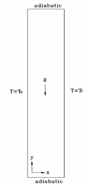
in Eq.(1)) is given in Choi and Lin[8]. The convection terms in theFig. 2 A schematic diagram of 1:5 rectangular cavity
LBM equations are treated by the second-order, central-difference scheme with a deferred correction method by Khosla and Rubin[16] to ensure the numerical stability.
(28) where the superscript
means the previous time step level and the subscript
implies the central-difference scheme.The test problem considered in the present study is a natural convection of air in a rectangular cavity with an aspect ratio of 1:5 as shown in Fig. 2. The height of the cavity is H=2.5m, the width of the cavity is L=0.5m and the temperature difference between the hot and cold walls is 45.8°K. The Rayleigh number based on the height of the cavity is Ra=4.3×10
10
and the Prandtl number is Pr=0.71. King[17] has carried out extensive measurements for this problem and his experimental data is reported in King[17] and Cheesewright et al.[18]. The experimental data by King[18] has a problem in that the top wall is not fully insulated. This makes the turbulence level near the hot wall high and that near the cold wall low, and this affects the distribution of the turbulence quantities in all the solution domain.Fig. 3 shows the comparison of the predicted results with the measured data for the vertical velocity component at y/H=0.5. As shown in the figures, the agreement
Fig. 3 Mean vertical velocity profiles at y/H=0.5
Fig. 4 Vertical velocity fluctuation profiles at y/H=0.5
between the measured data and both predictions are fairly good and there does not exist a visible difference between two predictions by LBM (FVLBM) and Navier-Stokes equation method (FVM). The elliptic-relaxation model by Medic and Durbin[10] with AFM predicts fairly well the mean velocity component and the turbulent quantities which will be shown in the subsequent figures.
Fig. 4 shows the comparison of the predicted vertical velocity fluctuation at a mid-height (y/H=0.5) with the experimental data. The experimental data shows a nearly symmetric profile, however, when one considers the insufficient insulation problem at the top wall, the measured data near the hot and cold walls are not correct.
Therefore, the magnitude of the experimental data near the hot wall should be greater than that near the cold wall.
Fig.5 Reynolds shear stress profiles at y/H=0.5
Fig. 6 Vertical turbulent heat flux profiles at y/H=0.5
The predictions follow the trend of the measured data well except for the central region of the cavity where the flow is weakly stratified. The two predictions slightly under-predict the vertical velocity fluctuation near the wall and over-predict it at the central region of the cavity.
The difference between two predictions is invisible.
Fig. 5 shows the profiles of the predicted Reynolds shear stress
at a mid-plane (y/H=0.5) of the cavity together with the measured data. The measured data shows clearly the insufficient insulation problem at the top wall. If we consider this problem, the present two methods fairly well predict the Reynolds shear stress
. The difference between two predictions is also invisible.Fig. 6 shows the profiles of the predicted vertical turbulent heat fluxes,
, at the mid-plane (y/H=0.5) ofFig. 7 Wall shear stress profile along the walls
Fig. 8 Local Nusselt number along the walls
the cavity with the measured data. It is noted that the vertical turbulent heat flux
plays a very important role in the dynamics of the turbulent kinetic energy in the buoyant turbulent flows and it directly influences the overall prediction of all the quantities. It is noted that the AFM contains all the temperature and mean velocity gradients together with a correlation between the gravity vector and temperature variance, as shown in Eq. (21).The elliptic-relaxation model with AFM predicts well the vertical turbulent heat flux near the hot wall region and this figure shows that the AFM is an accurate and stable model in the prediction of turbulent natural convection.
Fig. 7 and Fig. 8 show the comparisons of the predicted results with the measured data for the wall shear stress and the local Nusselt number at the hot wall
reported in King[17]. The two methods predict the wall shear stress at the walls very well and the smooth laminar to turbulent transition at the lower portion of the hot wall observed in the experimental data is also predicted well. It is noted that the measurement of the velocity components near the bottom wall is more accurate than that near the top wall due to an insufficient insulation at the top wall.
The present elliptic-relaxation model with AFM predicts accurately the local Nusselt number at the hot and cold walls, and the transition phenomenon at the lower portion of the hot wall is also predicted well. Compared to the other variables, the wall shear stress and the local Nusselt number are very sensitive due to the very fine grid near the walls. In the case of wall shear stress there exist a very small difference between two predictions. There is no difference between two methods in the prediction of the local Nusselt number at the walls.
4. C ONCLUSIONS
The finite-volume based LBM is formulated together with the HYBRID thermal model and is applied to the prediction of turbulent natural convection in a rectangular cavity. The elliptic-relaxation model with the algebraic heat flux model is employed for the turbulence model and this model predicts accurately the mean and turbulence quantities. There exists no visible difference in all the predicted results between the LBM and the Reynolds-averaged Navier-Stokes equation method except for the wall shear stress where a small difference is observed. These observations indicate that the LBM with the HYBRID thermal model is as accurate as the conventional Reynolds-averaged Navier-Stokes equation method and can be confidently applied to the predictions of various engineering turbulent natural convection problems.
A CKNOWLEDGEMENT
This study has been supported by the Nuclear Research and Development Program of the Ministry of Education, Science and Technology of Korea.
R EFERENCES
[1] 1998, Chen, S. and Doolen, G.D., "Lattice Boltzmann method for fluid flow," Annu. Rev. Fluid Mech., Vol.30, pp.329-364.
[2] 1993, Alexanders, F., Chen, S. and Sterling, J.,
"Lattice Boltzmann thermo-hydrodynamics," Phys. Rev.
E, Vol.47, pp.R2249-R2252.
[3] 1997, Shan, X., "Solution of Rayleigh Benard convection using a lattice Boltzmann method," Phys.
Rev. E, Vol.55, pp.2780-2788.
[4] 1998, He, X., Chenand S. and Doolen, G.D., "A novel thermal model for the lattice Boltzmann method in incompressible limit," J. Comput. Phys., Vol.146, pp.282-300.
[5] 2003, Peng, Y., Shu, C. and Chew, Y.T., "A 3D incompressible thermal lattice Boltzmann model and its application to simulate natural convection in a cubic cavity," J. Comput. Phys., Vol.193, pp.260-274.
[6] 2011, Choi, S.K. and Kim, S.O., "Comparative analysis of thermal models in the lattice Boltzmann method for the simulation of natural covection in a square cavity," Numer. Heat Transfer, B, Vol.60, pp.135-145.
[7] 1998, Teixeira, C.M., "Incorporating turbulence models into the lattice-Boltzmann method," Int. J. Modern
Phys. C, Vol.9, pp.1159-1175.
[8] 2010, Choi, S.K. and Lin, C.L., "A simple finite-volume formulation of the lattice Boltzmann method for laminar and turbulent Flows," Numer. Heat
Transfer, B, Vol.58, pp.242-261.
[9] 2004, Zhou, Y., Zhang, R., Staroselsky, I. and Chen, H., "Numerical simulation of laminar and turbulent buoyancy-driven flows using a lattice Boltzmann based algorithm," Int. J. Heat Mass Transfer, Vol.47, pp.4869-4879.
[10] 2002, Medic, G. and Durbin, P.A., "Toward Improved prediction of heat transfer on turbine blades," J.
Turbomachinery, Vol.124, pp.187-192.
[11] 2004, Choi, S.K., Kim, E.K. and Kim, S.O.,
"Computation of turbulent natural convection in a rectangular cavity with the
model,"Numer. Heat Transfer, Part B, Vol.45, pp.159-179.
[12] 1989, Ince, N.Z. and Launder, B.E., "On the computation of buoyancy-driven turbulent flows in rectangular enclosures," Int. J. Heat Fluid Flow, Vol.10, pp.110-117.
[13] 1995, Kenjeres, S. and Hanjalic, K., "Prediction of turbulent thermal convection in concentric and eccentric annuli," Int. J. Heat Fluid Flow, Vol.16, pp.428-439.
[14] 2008, Latt, J., Chopard, B., Malaspinas, D., Deville, M. and Michler, A., "Straight velocity boundaries in the lattice Boltzmann method," Phys. Rev. E, Vol.77, pp.056703-1~16.
[15] 1997, Zou, Q. and He, X., "On pressure and velocity boundary conditions for the lattice Boltzmann BGK model," Phys. Fluids, Vol.9, pp.1591-1598.
[16] 1974, Khosla, P.K. and Rubin, S.G., "A diagonally dominant second order accurate implicit scheme,"
Comput. Fluids, Vol.2, pp.207-209.
[17] 1989, King, K.V., "Turbulent natural convection in
rectangular air cavityies", Ph.D Thesis, Queen Mary College, University of London, UK.
[18] 1986, Cheesewright, R., King, K.J. and Ziai, S.,
"Experimental data for the validation of computer codes for the prediction of two-dimensional buoyant cavity flows," Proceedings of ASME Meeting, HTD, Vol.60, pp.75-86.