Econometric Estimation of the Climate Change Policy Effect in the U.S. Transportation Sector
Choi, Jaesung†
National Infrastructure Division, Korea Research Institute of Human Settlements, Korea
ABSTRACT
Over the past centuries, industrialization in developed and developing countries has had a negative impact on global warming, releasing CO2 emissions into the Earth’s atmosphere. In recent years, the transportation sector, which emits one-third of total CO2 emissions in the United States, has adapted by implementing a climate change action plan to reduce CO2 emissions. Having an environmental policy might be an essential factor in mitigating the man-made global warming threats to protect public health and the coexistent needs of current and future generations;
however, to my best knowledge, no research has been conducted in such a context with appropriate statistical validation process to evaluate the effects of climate change policy on CO2 emission reduction in recent years in the U.S. transportation. The empirical findings using an entity fixed-effects model with valid statistical tests show the positive effects of climate change policy on CO2 emission reduction in a state. With all the 49 states joining the climate change action plans, the U.S. transportation sector is expected to reduce its CO2 emissions by 20.2 MMT per year, and for the next 10 years, the cumulated CO2 emission reduction is projected to reach 202.3 MMT, which is almost equivalent to the CO2 emissions from the transportation sector produced in 2012 by California, the largest CO2 emission state in the nation.
Key words: Climate Change Policy, CO2, Entity Fixed-Effects Model, Heteroskedasticity and Autocorrelation- Consistent (HAC) Standard Errors, Transportation
1) Emissions and sinks regarding land use (e.g., deforestation) are not included (The United States Environmental Protection Agency, 2013).
†Corresponding author: [email protected]
Received November 22, 2016 / Revised December 7, 2016 1st, December 26, 2016 2nd / Accepted January 9, 2017
1. INTRODUCTION
The effects of global warming have been observed around the world in the form of more frequent wildfires, longer droughts, and stronger tropical storms, which can have negative impacts on the Earth’s societal, ecological, and environmental systems (The National Aeronautics and Space Administration, 2014). Carbondioxide (CO2) emissions contribute to global warming through the greenhousegas (GHG) effect by holding heat energy from the sun in the Earth’s atmosphere, producing increases in global average temperatures (The U.S. Environ- mental Protection Agency, 2015). The Intergovernmental Panel on Climate Change (2014) reported that CO2 accounted for 57% of total global GHG emissions in 2004 and was the largest
single source of emissions. They also reported that CO2 emi- ssions produced by the transportation sector accounted for as much as 13% of total global GHG emissions from the com- bustion of fossil fuel1).
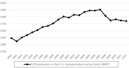
Among the five economic sectors in the U.S. (electricity, transportation, industry, commercial and residential, and other), CO2 emissions from the transportation sector ranked second highest, explaining 32% of total U.S. GHG emissions in 2012 (The U.S. Environmental Protection Agency, 2013). Although CO2 emissions from the transportation sector have increased, they reached a peak in 2007 (Fig. 1). Regarding the reduction after 2007, Choi et al. (2014) and Choi and Roberts (2015) suggested a couple of possible factors: 1) a government policy change (stricter federal regulations for GHG emissions) to-
2) “Light duty vehicles” refers to vehicles with a maximum gross vehicle weight rating of less than 8,500 pounds (TransportPolicy.net, 2013).
3) The extent of this study is limited to a macro analysis at this time, not by a state by state analysis, and thus the author focuses on major, middle, and minor groups after reviewing levels of CO2 emissions by state.
Fig. 1. CO2 emissions from the U.S. transportation sector, 1990 to 2012.
wards CO2 emission reduction, and 2) a decline in fuel con- sumption caused by higher oil prices led to increases fuel economy, production from alternative sources, and fewer miles travelled by light duty vehicles2).
For the last two decades, increasing interest in reducing CO2 emissions has generated numerous studies of the major CO2 emitting sectors (e.g., power, industry, transportation, etc.) mainly using the Laspeyres or the Divisia methods to attribute the growth in CO2 emissions to the potential driving forces. However, those methods are limited by their inability to consider the effects of qualitative factors, such as a change in environmental policy, while leaving to speculate the effects of an environmental policy change on CO2 emissions. In con- trast, other researchers have incorporated an environmental policy factor while studying CO2 emission changes in passenger transport, freight transport, transport land use, and highway accidents when focusing on forecasting CO2 emissions, the effects of an environmental policy change, or revealing the re- lationship between CO2 emissions and their potential driving factors (Diakoulaki et al., 2007; Al-Ghandoor et al., 2009;
Choi et al., 2010; Chung et al., 2013; Barido and Marshall, 2014; Kim et al., 2016; Park et al., 2016; Zhang et al., 2016).
Even though quantitative and qualitative analyses of CO2
emissions have been performed, to the best of my knowledge no research has been conducted with statistical validation process since 2007 to evaluate the effects of climate change policy on CO2 emissions produced by the U.S. transportation sector. Thus, the objectives of this study are to: I) identify whether climate change policies can reduce CO2 emissions from the U.S. transportation sector with appropriate statistical validation tools; ii) quantify the effects of U.S. climate change policy on CO2 emissions in the 49 contiguous U.S. states and for the nation 3); and iii) determine whether the effects of U.S.
climate change policy are consistent states. The findings of this study will be helpful to state and federal policy planners in evaluating the effects of climate change policy within their boundaries and nation wide and will provide a base on which to improve and accelerate the trend of CO2 emission reduction through the implementation of stricter environmental regula- tions all over the world.
2. BACKGROUND 2.1 Study Area
The World Bank (2015) defines the U.S. as a high-income country among the Organization for Economic Cooperation
and Development members, with gross national income per capita and total population of $53,470 and 319 million in 2014, respectively. In contrast, the U.S. transportation sector in 2011 emitted the largest CO2 emissions of 1,629 million metrictons (MMT) in the world, which was even higher than the summation of the European Union and China, the CO2
emissions of which were 1,535 MMT (=897+638) (The World Bank, 2015).
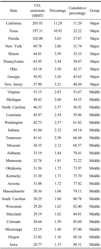
The CO2 emissions from the U.S. transportation sector during the study period of 2007∼2012 vary by state, but show three kinds of clusters, as presented in Table 1. The first one is the major CO2 emission group, which includes California, Texas, and Florida, the CO2 emissions of which contributed almost one-third of the total U.S. transportation CO2 emissions, and if the next 6l argest states (Florida, NewYork, Illinois, Pennsylvania, Ohio, Georgia, and NewJersey) are added, then they would account for almost 50% of the total U.S. trans- portation CO2 emissions. Second, the total CO2 emissions of the other next largest CO2 emission states, from Virginia to Kansas in Table 1, showing less than 3% but above 1% CO2
emissions in the total CO2 emissions, account for the other 40%
of the total CO2 emissions; for this reason, they were classified with the middle CO2 emission group. Third, forming the minor CO2 emission group, the rest of the states emitted less than 1% of the CO2 emissions, occupying the bottom 10% of CO2 emissions. Fig. 2 provides a geographic description of each group by state.
2.2 Air Pollution Regulations including a Climate Change Action Plan
The first federal act regarding air pollution was initiated with the Air Pollution Control Act of 1955 to protect public health from disease caused by air pollution. Congress enacted the Clean Air Act in 1970 to establish national air quality standards and made major revisions in 1977 and 1990. Since the 2000s, with the Energy Policy Act in 2005, Energy Inde- pendence and Security Act in 2007, and presidential procla- mations for CO2 emission reduction in recent years, the USEPA has established stricter air pollution regulations.
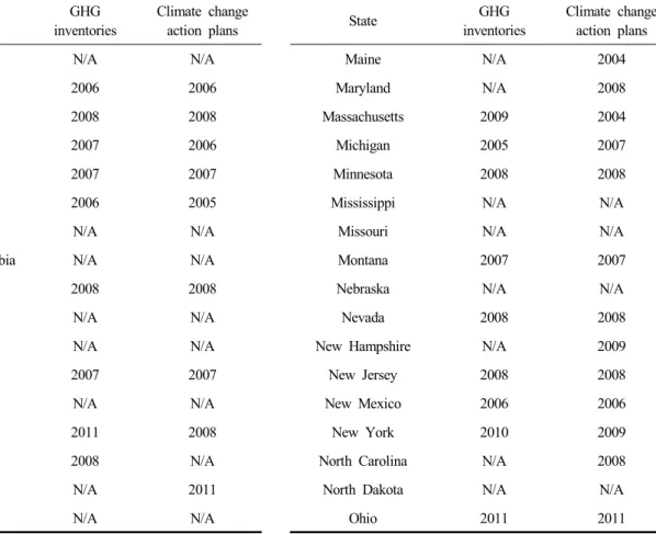
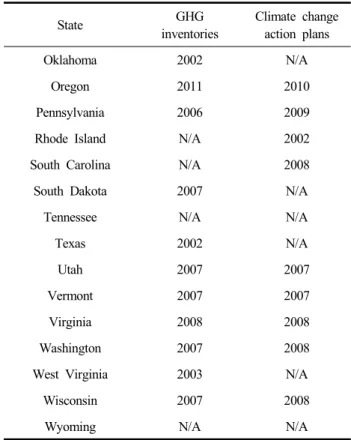
For the state-level climate change policy, Table 2 shows when the GHG inventory and/or climate change action plan was completed in each state. Of the 49 U.S. states, 31 (29)
Table 1. CO2 emissions by state, percentage and cu- mulative percentage of the total CO2 emissions from the U.S. transportation sector in 2012, and group classification
State
CO2
emissions (MMT)
Percentage Cumulative percentage Group
California 203.93 11.29 11.29 Major
Texas 197.31 10.93 22.22 Major
Florida 102.08 5.65 27.87 Major
New York 69.78 3.86 31.74 Major
Illinois 64.81 3.59 35.33 Major
Pennsylvania 63.95 3.54 38.87 Major
Ohio 63.18 3.50 42.37 Major
Georgia 58.92 3.26 45.63 Major
New Jersey 57.90 3.21 48.84 Major
Virginia 51.15 2.83 51.67 Middle
Michigan 48.43 2.68 54.35 Middle
North Carolina 46.33 2.57 56.92 Middle
Louisiana 45.87 2.54 59.46 Middle
Washington 42.73 2.37 61.82 Middle
Indiana 41.84 2.32 64.14 Middle
Tennessee 41.61 2.30 66.44 Middle
Missouri 38.35 2.12 68.57 Middle
Alabama 33.19 1.84 70.41 Middle
Minnesota 32.76 1.81 72.22 Middle
Oklahoma 31.56 1.75 73.97 Middle
Kentucky 31.30 1.73 75.70 Middle
Arizona 31.08 1.72 77.42 Middle
Massachusetts 30.36 1.68 79.11 Middle
South Carolina 30.25 1.68 80.78 Middle
Wisconsin 29.20 1.62 82.40 Middle
Maryland 29.19 1.62 84.01 Middle
Colorado 28.64 1.59 85.60 Middle
Mississippi 25.19 1.40 87.00 Middle
Oregon 21.02 1.16 88.16 Middle
Iowa 20.77 1.15 89.31 Middle
4) The independent variables examined are as follows: 1) all petroleum products consumed by the transportation sector; 2) all petroleum products’ average price in the transportation sector; 3) population; 4) GDP in the transportation sector; 5) number of employees working for the transportation sector; and 6) vehicle mileage traveled (VMT).
Table 1. Continued
State
CO2
emissions (MMT)
Percentage Cumulative percentage Group
Arkansas 19.32 1.07 90.38 Middle
Kansas 18.40 1.02 91.40 Middle
Utah 16.86 0.93 92.33 Minor
Connecticut 15.55 0.86 93.19 Minor
New Mexico 14.20 0.79 93.98 Minor
Nevada 14.04 0.78 94.76 Minor
Nebraska 13.76 0.76 95.52 Minor
West Virginia 11.75 0.65 96.17 Minor
North Dakota 9.22 0.51 96.68 Minor
Idaho 9.17 0.51 97.19 Minor
Wyoming 8.24 0.46 97.65 Minor
Maine 8.02 0.44 98.09 Minor
Montana 8.00 0.44 98.53 Minor
South Dakota 6.97 0.39 98.92 Minor
New Hampshire 6.88 0.38 99.30 Minor
Delaware 4.36 0.24 99.54 Minor
Rhode Island 3.87 0.21 99.76 Minor
Vermont 3.34 0.19 99.94 Minor
District of
Columbia 1.08 0.06 100.00 Minor
Notes: The CO2 emission data for 2012 were obtained from the U.S. Environmental Protection Agency (The United States Environmental Protection Agency, 2014); the total U.S.
CO2 emissions in 2012 for the 49 states were 1,838.71 MMT.
have completed a climate change action plan (GHG inventory) within their boundaries. A climate change action plan contains specific policy recommendations to address and reduce GHG emissions in various sectors, including transportation. Trans- portation-related emission reduction strategies are as follows:
Low carbon fuel standard, trip reduction programs, heavy-duty
vehicle anti-idling measures, clean vehicle purchase incentives, vehicle emissions standards, pay as you drive insurance, or others (Morrow et al., 2010; Choi and Roberts, 2014).
3. DATA AND METHODOLOGY
Various independent variables4) in the literature were taken into account to explain the factors of CO2 emission reduction in the transportation sector; therefore, the seven in dependent variables, including the implementation of a climate change policy, were all initially examined by a stepwise regression even though the effects of such apolicy are of primary interest in this study. The stepwise regression automatically selected the most important in dependent variables for modeling the mean dependent variable based on a t-test, and the brief pro- cedures used are explained as follows: 1) all possible one- variable models of a linear form were fitted; 2) the best two- variable model of the form was selected through there maining (k—1), where k is the number of independent variables; and 3) the researchers checked for the third independent variable and this process continued until further independent variables did not appear to contribute to a significant p-value with the variables already in the model (Mendenhall and Sincich, 2011).
After the procedures, the four independent variables (fuel consumption, regulation of CO2 emissions, VMT, and GDP in the transportation sector, ordered by the lower p-value and statistically significant at the 10% level) remained. However, due to the high possibility of multicollinearity between the four variables, the variance inflation factor (VIF) was tested for each variable. Excluding the regulation of CO2 emissions, the three variables were highly correlated, showing a VIF greater than 10 (Mendenhall and Sincich, 2011); thus, only the variable of fuel consumption, which is directly connected to CO2 emissions, remained and the others were dropped.
Finally, the two independent variables (fuel consumption and regulation of CO2) were selected. The former variable was obtained from the online data base of the U.S. Energy Infor- mation Administration (2015) and was measured in billion Btu. The latter variable was produced through a qualitative
Fig. 2. Study area by groups.
Table 2. GHG inventories and climate change action plans by state
State GHG
inventories
Climate change action plans
Alabama N/A N/A
Arizona 2006 2006
Arkansas 2008 2008
California 2007 2006
Colorado 2007 2007
Connecticut 2006 2005
Delaware N/A N/A
District of Columbia N/A N/A
Florida 2008 2008
Georgia N/A N/A
Idaho N/A N/A
Illinois 2007 2007
Indiana N/A N/A
Iowa 2011 2008
Kansas 2008 N/A
Kentucky N/A 2011
Louisiana N/A N/A
Table 2. Continued
State GHG
inventories
Climate change action plans
Maine N/A 2004
Maryland N/A 2008
Massachusetts 2009 2004
Michigan 2005 2007
Minnesota 2008 2008
Mississippi N/A N/A
Missouri N/A N/A
Montana 2007 2007
Nebraska N/A N/A
Nevada 2008 2008
New Hampshire N/A 2009
New Jersey 2008 2008
New Mexico 2006 2006
New York 2010 2009
North Carolina N/A 2008
North Dakota N/A N/A
Ohio 2011 2011
Table 2. Continued
State GHG
inventories
Climate change action plans
Oklahoma 2002 N/A
Oregon 2011 2010
Pennsylvania 2006 2009
Rhode Island N/A 2002
South Carolina N/A 2008
South Dakota 2007 N/A
Tennessee N/A N/A
Texas 2002 N/A
Utah 2007 2007
Vermont 2007 2007
Virginia 2008 2008
Washington 2007 2008
West Virginia 2003 N/A
Wisconsin 2007 2008
Wyoming N/A N/A
Notes: Information was obtained from the U.S. Environmental Protection Agency (The United States Environmental Pro- tection Agency, 2014); N/A means that a state has not completed a GHG inventory or a climate change action plan.
variable technique based on information regarding a climate change action planfrom Table 2. For the dependent variable, CO2 emissions were derived from the USEPA and measured in MMT (The U.S. Environmental Protection Agency, 2014).
All the data ranged from 2007 to 2012 by state.
An entity fixed-effects panel regression model was utilized to estimate the effects of climate change policy on CO2 emi- ssion reduction in the U.S. transportation sector. The empirical econometric model for the pooled data and each group is as follows (Pindyck and Rubinfeld, 1997; Stock and Watson, 2011):
yit = β0+β1X1it+β2X2it+y3D2i+y4D3i+…+yn+1Dni+uit (1) where, β0, β1, β2, y3, …, yn+1 are unknown coefficients; X1it
is the implementation of a climate change policy by state i in year t; X2it is the transportation sector fuel consumption by state i in year t; D2i is a qualitative variable that equals 1 when i = 2 and 0 otherwise; D3i is a qualitative variable that equals 1 when i = 3 and 0 otherwise, and so on; uit and is an error term.
n—1 qualitative variables were used to avoid the dummy variable trap by omitting the first qualitative variable, D1i. The rest of the qualitative variables take care of the effects of all the omitted variables that are not the same from each state to another but are constant over time. To summarize, the proce- sses of the model performed in this study are as follows. First, the author extracted the appropriate regressors for the model by the stepwise regression and multicollinearity test. Second, the author tested whether the entity fixed-effects regression model is the best among other possible panel models, such as the time fixed effects, one-way random effects, and two-way random effects, by using F statistics and comparing the overall model fit and the estimated coefficients’ statistical significance.
Third, a couple of statistical tests for verifying the serial co- rrelation and heteroskedasticity were processed by the Durbin- Watson test and the Breusch-Pagan test, and the problems found were fixed by heteroskedasticity and autocorrelation- consistent (HAC) standard errors. Fourth, the author regressed the panel model and then analyzed the regression results based on the estimated coefficients’ p-values at the 10%, 5%, and 1% significance levels.
4. EMPIRICAL RESULTS
The empirical findings regarding the effects of climate chan- ge policy on CO2 emission reduction in the U.S. transporta- tion sector from 2007 to 2012 are summarized in two parts- pooled data and each group-in Table 3 and Table 4. In both tables, the F statistic’s null hypothesis, which is no fixed effects, was rejected at the 1% level of significance. A couple of OLS regression assumptions were tested and the test results are shown with the existence of positive serial correlation and he- teroskedasticity since the Durbin-Watson tests were less than 2 and the null hypothesis of homoskedasticity in the Breusch- Pagan tests were rejected at the 5% significant level, respec- tively.
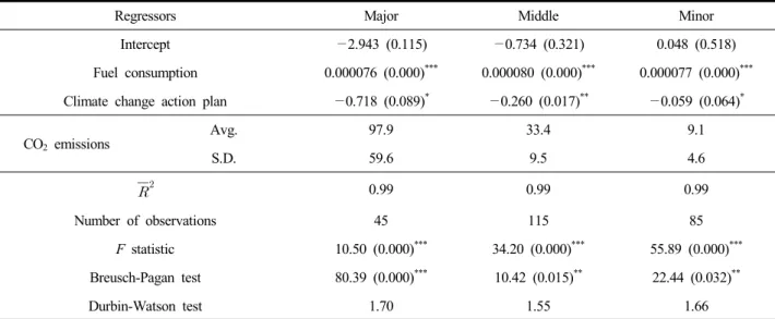
Table 4. Regression results for each group
Regressors Major Middle Minor
Intercept —2.943 (0.115) —0.734 (0.321) 0.048 (0.518)
Fuel consumption 0.000076 (0.000)*** 0.000080 (0.000)*** 0.000077 (0.000)***
Climate change action plan —0.718 (0.089)* —0.260 (0.017)** —0.059 (0.064)*
CO2 emissions
Avg. 97.9 33.4 9.1
S.D. 59.6 9.5 4.6
0.99 0.99 0.99
Number of observations 45 115 85
F statistic 10.50 (0.000)*** 34.20 (0.000)*** 55.89 (0.000)***
Breusch-Pagan test 80.39 (0.000)*** 10.42 (0.015)** 22.44 (0.032)**
Durbin-Watson test 1.70 1.55 1.66
Notes: *,** and *** indicate significance at the 10%, 5%, and 1% level, respectively; the p-values are in parenthesis. The coefficients on all the cross-sectional dummies and control variables have been omitted. The null hypothesis of the Breusch-Pagan test is homoskedasticity, and the F statistic’s null hypothesis is no fixed effects.
5) The two control variables represent the U.S. economic recessions from 2007 to 2009 and the technological advancements for fuel economy in vehicle fleets. The variable of the U.S. economic recessions was constructed using a qualitative variable technique.
The variable of advances in fuel efficiency was constructed using the summation of vehicles sold in the U.S. from electric hybrid vehicles, flex-fuel vehicles on E85, and hydrogen vehicles and was obtained from the online database of the USEIA (The United States Energy Information Administration, 2013).
Table 3. Regression results for the entire U.S Regressors Coefficients and p-values
Intercept —1.537 (0.064)*
Fuel consumption 0.000077 (0.000)***
Climate change action plan —0.413 (0.002)***
0.99
Number of observations 245
F statistic 20.01 (0.000)***
Breusch-Pagan test 80.39 (0.000)***
Durbin-Watson test 1.74
Notes: *,** and *** indicate significance at the 10%, 5%, and 1%
level, respectively. The coefficients on all the cross-sec- tional dummies and control variables have been omitted.
The null hypothesis of the Breusch-Pagan test is homo- skedasticity, and the F statistic’s null hypothesis is no fixed effects.
To address these problems, HAC standard errors were used in the entity fixed-effects models. The HAC standard errors functioned to make the regression errors remain randomly correlated within a grouping and uncorrelated across groups (Stock and Watson, 2011). Additionally, to consider the poten- tial omitted variable bias arising from omitting both technolo- gical advancements in fuel efficiency and the U.S. economic recession, the two control variables5) were utilized in the re- gression models. The concept of a control variable replaced the first least squares assumption of exogeneity with conditional mean in dependence6) to prevent the estimated causal effect of interest from suffering from endogeneity (Wooldridge, 2012).
As Stock and Watson (2011) explained in 2011, this study distinguished between regressors for which we have an inte- rest in estimating a causal effect and a control variable. By establishing the alternative assumption, “the OLS estimator of the effect of interest was unbiased, but the OLS coefficients on control variables were in general biased and did not have
6) Conditional mean independence is mathematically shown with the equation E(ui∣X1i, X2i) = E(ui∣X2i), where X1i is the variable of interest, X2i is the control variable, and ui is the error term. Including X2i makes X1i uncorrelated with ui, and therefore OLS can be used to estimate the effect on Yit of a change in X1i [65].
7) The states that have not implemented any climate change action plans are as follows: Georgia and Texas in the major group and Alabama, Indiana, Louisiana, Mississippi, Missouri, Oklahoma, and Tennessee in the middle group.
a causal interpretation” (Stock and Watson, 2011, p. 231).
In Table 3, an overall effect of a climate change action plan on CO2 emission reduction in the U.S. transportation sector across the 49 U.S. states was estimated and its coefficient shows a negative value of —0.413. If a state’s policy plan of CO2 emi- ssion reduction took effect during the period of 2007∼2012, then it on average has reduced the CO2 emissions per year by 0.413 MMT. Since the 31 states have completed such a CO2
emission reduction policy plan through a climate change action plan, their total reduced CO2 emissions reached 12.803 MMT in 2012, which was bigger than the entire transportation CO2
emissions of West Virginia in 2012, 11.75 MMT. As the author expected, the fuel consumption in the transportation sector has had a positive impact on CO2 emissions, technically 1 billion Btu in fuel consumption by transport in a state per year on average, increasing the CO2 emissions by 0.000077 MMT.
Table 4 provides the effects of the climate change policy on CO2 emission reduction in the three groups. Overall, the stability of average and standard deviation of CO2 emission by each group would not seem to be deteriorated when considering the difference of the levels of CO2 emission. The major group shows the most significant CO2 emission reduction through the climate change action plan, followed by the middle and minor groups. The policy plan of CO2 emission reduction in a state in the major group on average has almost three times as po- werful a CO2 emission reduction effect than that of the middle group, while a state in the minor group has on average only one-tenth of the CO2 emission reduction effect compared with the major group. Since a climate change action plan exerts di- fferent effects within the groups, if the time and financial re- sources available are limited in the nation, then it is recommend to focus on letting the federal government first support the states in the major and middle groups7) rather than the minor group.
5. CONCLUSIONS
The human activities for industrialization have been acce-
lerating and raising the global temperature for centuries, due to the increasing CO2 emissions released into the atmosphere by most of the economic sectors in a nation. As a result, we are unexpectedly experiencing severe natural disasters in many areas worldwide more frequently than in the past and thereby more people are being exposed to danger to their life and property.
A positive environmental policy change will be an essential factor in protecting public health and the coexistent needs of current and future generations; as Benjamin Franklin (Sussman, 2006) emphasized in 1963 at the University of North Dakota, the environment is an important public policy concern. In the U.S., such a change to relax the current high-level global war- ming and reverse it to a moderate level of around 1990 has been evident in various social and economic sectors; among them, the transportation sector, which emits one-third of the total CO2 emissions in the U.S., has been quickly adapting by implementing a climate change action plan to reduce its CO2
emissions.
This study revealed how effectively a climate change policy can function in the U.S. transportation sector by estimating the quantified climate change policy impacts not only for the na- tional level, but also for the major, middle, and minor CO2
emission groups. The empirical findings using an entity fixed- effects model with various valid statistical tests shows an evi- dently positive effect of the existence of a climate change policy in a state on decreasing its CO2 emissions, even in the case of the minor CO2 emission group. If all of the 49 states can implement climate change action plans, the U.S. transportation sector can reduce its CO2 emissions by 20.2 MMT per year, and for the next 10 years, the cumulated CO2 emission reduction will reach 202.3 MMT, which is almost equivalent to the CO2
emissions produced by the transportation sector in 2012 in Ca- lifornia, the largest CO2 emitting state in the nation. All of this finally suggests the importance of implementing a climate change policy to reduce CO2 emissions in the transportation sector.
6. STUDY LIMITATION
The author tried to find out scientific proofs regarding im- plementing effective climate change policies in the transpor- tation sector as using an econometric tool which was well known in the econometrics. We probably think that decrease of fuel consumption will step out of CO2 emissions in the air more and more, but regardless of intuitive awareness, evident proofs need to be revealed. In this study, the author macrosco- pically found out the CO2 reduction effect of climate change policies, but in the next study microscopic effects of each cli- mate change policy needs to be reviewed for the detailed policy effect analysis.
ACKNOWLEDGEMENT
This study was supported by the Korea Research Institute for Human Settlements basic research. The contents are sole responsibility of the author. The author would like to thank colleagues in the institute and anonymous reviewers for their constructive comments.
REFERENCES
Al-Ghandoor A, Jaber JO, Samhouri M, Al-Hinti I. 2009.
Analysis of aggregate electricity intensity change of the Jordanian industrial sector using decomposition technique.
International Journal of Energy Research 33:255-266.
Barido DP, Marshall JD. 2014. Relationship between urbani- zation and CO2 emissions depends on income level and policy. Policy Analysis 48:3632-3649.
Choi M, Kim J, Lee HJ, Jang YK. 2010. Estimation of green- house gas emission from off-road transportation. Journal of Climate Change Research 1:211-217.
Choi J, Roberts DC. 2015. How does the change of carbon dioxide emissions change affect transportation producti- vity? A case study of the U.S. transportation sector from 2002 to 2011. Open Journal of Social Science 3:96-106.
Choi J, Roberts DC, Lee E. 2014. Forecast of CO2 emi- ssions from the U.S. transportation sector: Estimation from a double exponential smoothing model. Journal of Transportation Research Forum 53:63-81.
Chung Y, Cho H, Choi K. 2013. Impacts of freeway acci- dents on CO2 emissions: A case study for Orange County, California, US. Transportation Research Part D 24:120- 126.
Diakoulaki D, Mavrotas G, Orkopoulos D, Papayannakis L.
(2006). A bottom-up decomposition analysis of energy- related CO2 emissions in Greece. Energy 31:2638-2651.
Intergovernmental Panel on Climate Change. 2014. Climate Change 2014: Impacts, adaptation, and vulnerability. Re- trieved January 5, 2015, from http://www.ipcc.ch/report/
ar5/wg2/
Kim M, Yoon YJ, Han J, Lee HS, Jeon EC. 2016. Analysis of GHG reduction potential on road transportation sector using the LEAP model. Journal of Climate Change Re- search 7:85-93.
Mendenhall W, Sincich T. 2011. A second course in statis- tics: Regression analysis. Pearson, London.
Morrow WR, Gallagher KS, Collantes G, Lee H. 2010. Ana- lysis of policies to reduce oil consumption and green- house-gas emissions from the US transportation sector.
Energy Policy 38:1305-1320.
Pindyck RS, Rubinfeld DL. 1997. Econometric models and economic forecasts. McGraw-Hill, New York.
Park YS, Lim SH, Egilmez G, Szmerekovsky J. 2016. Envi- ronmental efficiency assessment of US transport sector:
A slack-based data environment analysis approach. Trans- portation Research Part D: Transport and Environment.
Stock JH, Watson MW. 2011. Introduction to econometrics.
Addison-Wesley, Boston.
Sussman G. 2006. The Environment as an important public policy Issue. Retrieved January 9, 2015, from http://ww2.
odu.edu/ao/instadv/quest/Environment.html
The National Aeronautics and Space Administration. 2014.
The current and future consequences of global change.
Retrieved January 5, 2015, from http://climate.nasa.gov/
effects/
The United States Energy Information Administration. 2013.
Alternative Fuel Vehicle Data. Retrieved January 7, 2015, from http://www.eia.gov/renewable/afv/users.cfm#
tabs_charts-2
The United States Environmental Protection Agency. 2013.
Global greenhouse gas emissions data. Retrieved January
5, 2015, from http://www.epa.gov/climatechange/ghgemi- ssions/global.html
The United States Environmental Protection Agency. 2014.
Greenhouse gas inventory data explorer. Retrieved Janu- ary 3, 2015, from http://www.epa.gov/climatechange/ghg- emissions/inventoryexplorer/#transportation/allgas/source/
all
The United States Environmental Protection Agency. 2015.
Climate change & air quality. Retrieved January 5, 2015, from http://www.epa.gov/airquality/airtrends/2011/report/
climatechange.pdf
The World Bank. 2015. CO2 emissions from transport. Re- trieved January 6, 2015, from http://data.worldbank.org/
indicator/EN.CO2.TRAN.MT/countries?display=graph Wooldridge JM. 2012. Introductory econometrics: A modern
approach. Cengage Learning, Boston.
Zhang H, Chen W, Huang W. 2016. TIMES modelling of transport sector in China and USA: Comparisons from a decarbonization perspective, Apllied Energy 162:1505- 1514.