Accuracy Comparison of Air Temperature Estimation using Spatial Interpolation Methods according to Application of Temperature Lapse Rate Effect

(1)

†Corresponding author : E-mail: [email protected]

접수일자: 2014. 10. 20 / 수정일자: 2014. 11. 28 / 채택일자: 2014. 12. 10

기온감률 효과 적용에 따른 공간내삽기법의 기온 추정 정확도 비교 Accuracy Comparison of Air Temperature Estimation using

Spatial Interpolation Methods according to Application of Temperature Lapse Rate Effect

김용석․심교문^†․정명표․최인태 국립농업과학원 농업환경부 기후변화생태과

Kim, Yong Seok, Shim, Kyo Moon^†, Jung, Myung Pyo and Choi, In Tae Climate Change & Agroecology Division, National Academy of

Agricultural Science, Wanju, Korera

ABSTRACT

Since the terrain of Korea is complex, micro- as well as meso-climate variability is extreme by locations in Korea. In particular, air temperature of agricultural fields is influenced by topographic features of the surroundings making accurate interpolation of regional meteorological data from point-measured data.

This study was carried out to compare spatial interpolation methods to estimate air temperature in agricultural fields surrounded by rugged terrains in South Korea. Four spatial interpolation methods including Inverse Distance Weighting (IDW), Spline, Ordinary Kriging (with the temperature lapse rate) and Cokri- ging were tested to estimate monthly air temperature of unobserved stations. Monthly measured data sets (minimum and maximum air temperature) from 588 automatic weather system(AWS) locations in South Korea were used to generate the gridded air temperature surface. As the result, temperature lapse rate im- proved accuracy of all of interpolation methods, especially, spline showed the lowest RMSE of spatial interpolation methods in both maximum and minimum air temperature estimation.

Key words : Spatial Interpolation, IDW, Kriging, Spline, Air Temperature

1. 서론

우리나라의 지형은 복잡하여 국지적으로 다양한 기상 패턴을 나타나고 있지만, 한정적인 지역에만 기상관측장비가 설치되어 있어 모든 지역의 기상정 보를 얻기가 힘든 상황이다. 그렇기 때문에 농업분

야에서는 작물이 자라고 있는 지역이 아닌 기상관 측장비가 설치가 된 인근지역의 기상자료를 이용하 여 작물의 생육상황을 파악해야 한다. 이러한 문제 는 농업 정책자에게는 정확한 농산물의 생산량을 파악하기 힘들게 하여 농업정책을 실행하기 어렵게 하며, 농업인에게는 기상에 의해 발생한 피해에 대

(2)

해 정확한 이유를 파악하기 힘들게 만든다. 이런 상황을 해결하기 위한 방법 중에 역거리가중(Inver- se Distance Weighting; IDW), 크리깅(Kriging), 스플 라인(Spline)과 같은 공간내삽기법을 이용한 기상정 보의 상세화 연구가 수행되고 있으며, 최근에는 단 순히 공간내삽기법 만을 이용할 시에 생기는 문제 점을 극복하기 위한 연구도 함께 이루어지고 있다.

그 예로서, Yun et al.(2001)은 고도편차에 따른 기 온감률 효과를 고려한 역거리가중을 이용하여 기온 값을 추정한 연구를 수행하였으며, Chung et al.

(2002)은 기온감률뿐만 아니라, 냉기침강효과까지 고 려하여 기온값을 추정한 연구를 수행하였다. 그리 고 Lu and Wong(2008)은 역거리가중을 바탕으로 한 관측지점들이 군집되어 있는 정도에 따라 가중 치를 달리 주는 AIDW(Adaptive Inverse Distance Weighting)을 이용하여 강수량을 추정하였으며, Park and Jang(2008)은 이차변수로서 해발고도를 적용한 공동크리깅(Cokriging)을 이용하여 기온과 강수량을 추정하는 연구를 수행하였다.

본 연구에서는 기온값 추정에 있어서 여러 공간 내삽기법의 정확도를 비교하고, Yun et al.(2001)에 서 사용된 기온감률 효과를 적용에 따른 기온 추정 값의 정확도 변화를 비교하여 가장 오차가 작은 공 간내삽기법을 살펴봄과 아울러, 앞으로 수행해야 할 기상정보의 상세화 연구의 기초자료로 활용하기 위하여 수행하였다.

2. 재료 및 방법

2.1 가상자료 수집

국립농업과학원과 기상청에서 운영 중인 588지 점의 자동기상관측시스템(Automatic Weather Sta- tion: AWS)의 2012년도 일별 최고기온과 최저기온 을 수집하여 월 평균최고기온과 평균최저기온으로 계산하였다. 월 평균최고기온과 평균최저기온을 추 정하기 위하여 456지점을, 추정값을 검증하기 위하 여 132지점을 이용하였다.

2.2 공간내삽기법의 개요

2.2.1 역거리가중(Inverse Distance Weighting;

IDW)

추정값을 알고자 하는 미관측지점이 관측지점에 거리상 근접한 지점일수록 높은 가중치를 부여하 고, 멀어질수록 가중치를 낮게 부여하는 것을 기본 원리로 하는 기법이다(Cho and Jeong, 2006).

_

  



__

(1a)

_ 

  



_^{ }

(1b) 여기서, _는 추정값, _는 관측값, _는 가중치,

은 자료의 총수, 는 관측지점과 미관측 지점의 거리, 는 가중정도를 나타내는 계수이다.

2.2.2 크리깅(Kriging)

크리깅은 미관측지점의 값을 공간적인 상호관계 를 가지는 확률 변수의 가중 선형조합으로 유추되 는 기법으로(Goovaerts, 1997), 계산식은 식 (1a)과 같으며, 가중치 _는 예측값과 참값 사이의 오차분 산이 최소가 되도록 한다. 공간내삽 과정에서는 여 러 지점의 관측 값들을 통해 경험적 배리오그램을 구하며, 이것을 이용하여 정형화된 이론적 배리오 그램을 추정하게 된다. 배리오그램은 식 (2)와 같 이, 일정한 분리거리(lag)만큼 떨어진 값들의 차이 의 제곱의 평균을 나타내며, 일반적으로 분리거리 가 증가할수록 분산의 정도인 배리오그램은 증가하 게 된다(Choi, 2007).

  

 

  



 _   _ ^

(2) 여기서, 는 관측 값, 는 지연거리, 는 자료쌍의 총수를 나타낸다.

정규크리깅은 식 (3a)와 같이 예측오차를 최소로 하면서 가중치의 합이 1이라는 불편향의 제약조건 을 추가시킨 기법이며(Park and Jang, 2008), 공동크 리깅은 식 (3b)와 같이 두 가지 이상의 변수의 선

(3)

형조합을 사용하여 자료가 알려지지 않은 지점에서 값을 예측하는 기법이다. 이때, 공동크리깅에서는 예측하고자 하는 변수를 주변수라 하고, 주 변수가 아닌 이차 변수는 여러 개가 될 수 있다(Choi, 2007).

__{  }^ ^^^^^_{  }^ ^^^{ } (3a)

_

  



__

  



  



___

(3b) 여기서, _는 추정값, _는 주변수, _는 가중치,

는 사용된 주변수의 총자료수, _는 사용된 이차 변수의 총개수, _는 j번째 이차변수, _는 j번째 이차변수의 총자료수, _는 각 자료의 위치를 나타 낸다.

2.2.3 스플라인(Spline)

스플라인은 방사기반함수(RBF: Radial Basis Func- tion)로도 알려져 있으며, 관측된 지점의 값을 통과 하는 표면 곡률의 총합이 최소가 되게 표면을 형성 하여 미관측지점의 값을 예측하는 기법이다(Ster- ling, 2003; Kim et al., 2011).

2.3 기온감률

연중 날짜에 따른 기온감률을 주기함수로 표현 하면, 최고기온을 추정할 경우는 식 (4a)로, 최저기 온을 추정할 경우는 식 (4b)를 사용하여 기온감률 을 구한다(Yun et al., 2001).

  cos   (4a)

  cos   (4b) 여기서, 는 Julian day(1월 1일=1 , … , 12월 31 일=365)를 나타낸다.

2.4 공간내삽기법의 적용

역거리가중을 수행하기 위하여 가중계수(p)는 2 로 설정하였고, 내삽을 위해 사용한 지점 수는 3지 점으로 하였다. 정규크리깅과 공동크리깅을 수행하

기 위한 이론적 배리오그램은 가우스모형 식 (5a) 와 지수모형 식 (5b)로 설정하였다.

 __ _^

_{  exp}^{ }^

^^

(5a)

 _Exp_ _^



_{  exp}^{ }

^

(5b) 여기서, _는 문턱값, 는 분리거리, 는 상관거 리를 나타낸다(Choi, 2007).

역거리가중, 정규크리깅, 스플라인에 고도편차에 따른 기온감률을 적용하기 위해 270m DEM(Digital Elevation Model)을 이용하였고, 공동크리깅은 이차 변수로서 해발고도값을 적용하였다. 고도보정(공간 내삽기법에 의해 추정된 고도와 실제고도와의 편차 에 따른 기온감률)을 계산하기 위하여 Yun et al.

(2001)에서 사용한 식 (6a)를 기본으로 하였으며, 식 (6b)와 같이 각 공간내삽기법을 이용하여 해발고도 차에 따른 기온감률 효과를 계산하였다.







^{  }__

_^



^_





_ 





^

(6a)

  ^ (6b) 여기서, 는 DEM의 고도, ^는 역거리가중과 스 플라인, 정규크리깅을 이용하여 계산된 고도, 는 기온감률이다.

모든 계산 과정은 ArcGis 9.3의 ArcMap의 Geo- statistical Analyst와 Raster Calculator를 이용하였으 며, 270 m 해상도로 추정값을 산출하였다.

2.5 추정값 검증

각 공간내삽기법의 월 평균최고기온과 평균최저 기온의 관측값과 추정값의 오차를 비교하기 위하여 식 (7)과 같이 RMSE(Root Mean Square Error)를 계 산하였다.

RMSE=^^^^  ^



_ _^^ (7)

(4)

여기서, 는 관측값, ^는 추정값을 나타낸다.

3. 결과 및 고찰

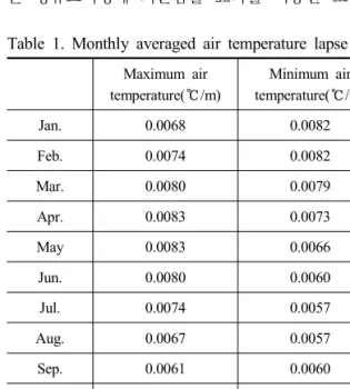
식 (4a)와 식 (4b)를 이용하여 계산한 최고기온과 최저기온의 일별 기온감률을 이용하여 월평균값으 로 계산한 결과 Table 1과 같이 나타났다. 최고기온 의 경우 4월과 5월에 고도에 따른 기온의 변화가 가장 큰 것으로 나타났고, 최저기온의 경우 1월과 2월에 가장 변화가 큰 것으로 나타났다.

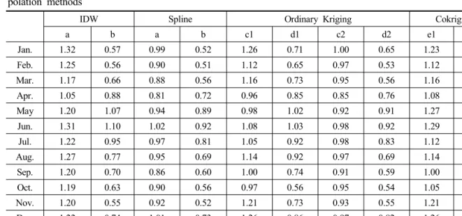
월별 평균최고기온 추정값의 RMSE를 비교하였 을 때 기온감률 효과를 적용하기 전에는 역거리가 중, 스플라인, 정규크리깅 추정값의 평균 RMSE가 0.93∼1.22 범위로 나타났으나, 적용한 후에는 0.67

∼0.81 범위로 나타나 모든 공간내삽기법에서 RM- SE가 낮아졌으며, 평균 RMSE는 기온감률 효과를 적용한 스플라인이 가장 낮게 나타났다(Table 2).

정규크리깅과 공동크리깅을 비교하였을 때 배리오 그램을 가우스모형으로 적용하였을 때보다 지수모 형으로 적용하였을 때 평균 RMSE가 더 낮게 나타 났으며, 고도를 이차변수로 이용한 공동크리깅보다 는 정규크리깅에 기온감률 효과를 적용한 모형의

Table 1. Monthly averaged air temperature lapse rate Maximum air

temperature(℃/m)

Minimum air temperature(℃/m)

Jan. 0.0068 0.0082

Feb. 0.0074 0.0082

Mar. 0.0080 0.0079

Apr. 0.0083 0.0073

May 0.0083 0.0066

Jun. 0.0080 0.0060

Jul. 0.0074 0.0057

Aug. 0.0067 0.0057

Sep. 0.0061 0.0060

Oct. 0.0058 0.0066

Nov. 0.0058 0.0073

Dec. 0.0062 0.0079

평균 RMSE가 더 낮게 나타났다.

월별 평균최저기온 추정값의 RMSE를 비교하였 을 때 기온감률 효과를 적용하기 전에는 역거리가 중, 스플라인, 정규크리깅에 의한 추정값의 경우 평 균 RMSE가 1.23∼1.53 범위로 나타났으나, 기온감 률 효과를 적용한 후에는 0.93∼1.19 범위로 나타 나, 최고기온의 경우와 동일하게 모든 공간내삽기 법에서 평균 RMSE가 낮아졌으며, 평균 RMSE는 기온감률 효과를 적용한 스플라인이 가장 낮게 나 타났다(Table 3). 크리깅의 비교에서도 최고기온의 결과값과 유사하게 배리오그램을 가우스모형으로 적용하였을 때보다 지수모형으로 적용하였을 때 정 확도가 더 높게 나타났으며, 공동크리깅보다 정규 크리깅에 기온감률 효과를 적용한 모형이 정확도가 더 높게 나타났다.

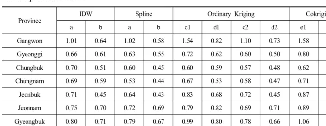
지역별로 RMSE를 비교한 결과(Table 4 and Ta- ble 5)에서는 모든 공간내삽기법에서 강원도가 다 른 지역에 비해 기온감률 효과를 적용한 후에 추정 값의 RMSE가 가장 크게 감소한 것으로 나타났는 데, 이는 상대적으로 강원도가 산지가 많기 때문인 것으로 예상된다.

본 연구에서 미관측지점의 최고기온과 최저기온 의 추정을 위하여 다양한 공간내삽기법과 기온감률 효과를 이용하여 정확도를 비교해 보았다. 우리나 라의 경우 지형의 굴곡이 심하기 때문에, 단순히 공간내삽기법만으로 추정한 값보다 해발고도에 따 른 기온감률 효과를 적용하였을 때가 월별 평균최 고기온의 경우, 역거리가중은 37%, 스플라인은 28

%, 정규크리깅(가우스모형)은 26%, 정규크리깅(지수 모형)은 27% 정도 정확도가 향상되는 것으로 나타 났으며, 월별 평균최저기온의 경우, 역거리가중은 28%, 스플라인은 25%, 정규크리깅(가우스모형)은 22

%, 정규크리깅(지수모형)은 23% 정도 정확도가 향 상되는 것으로 나타났다. 그리고 최종적으로 각 기 법의 평균 RMSE를 비교한 결과에서는 기온감률 효과를 적용한 스플라인이 최고기온의 경우 0.67이 고, 최저기온의 경우 0.93로 가장 낮게 나타났다.

비록, 본 연구에서는 스플라인을 이용한 기온 추 정값이 가장 RMSE 낮게 나타났지만, Anderson (2002)

(5)

Table 2. Comparison of RMSEs of monthly mean maximum air temperature estimated by four spatial interpolation methods

IDW Spline Ordinary Kriging Cokriging

a b a b c1 d1 c2 d2 e1 e2

Jan. 1.32 0.57 0.99 0.52 1.26 0.71 1.00 0.65 1.23 1.00

Feb. 1.25 0.56 0.90 0.51 1.12 0.65 0.97 0.53 1.12 0.97

Mar. 1.17 0.66 0.88 0.56 1.16 0.73 0.95 0.56 1.16 0.95

Apr. 1.05 0.88 0.81 0.72 0.96 0.85 0.85 0.76 1.08 0.85

May 1.20 1.07 0.94 0.89 0.98 1.02 0.92 0.91 1.27 0.93

Jun. 1.31 1.10 1.02 0.92 1.08 1.03 0.98 0.92 1.29 0.98

Jul. 1.22 0.95 0.97 0.81 1.05 0.92 0.98 0.83 1.12 0.97

Aug. 1.27 0.77 0.95 0.69 1.14 0.92 0.97 0.69 1.14 0.97

Sep. 1.20 0.70 0.86 0.60 1.00 0.74 0.91 0.59 1.00 0.90

Oct. 1.19 0.63 0.90 0.56 0.97 0.56 0.95 0.54 1.05 0.95

Nov. 1.20 0.55 0.92 0.52 1.21 0.73 0.93 0.55 1.21 0.93

Dec. 1.22 0.74 1.01 0.73 1.26 0.86 0.97 0.82 1.26 0.97

Avg. 1.22 0.77 0.93 0.67 1.10 0.81 0.95 0.70 1.16 0.95

a: no use temperature lapse rate, b: use temperature lapse rate, c1: no use temperature lapse rate and gauss model as variogram model, d1: no use temperature lapse rate and exponential model as variogram model, c2: use temperature lapse rate and gauss model as variogram model, d2: use temperature lapse rate and exponential model as variogram model, e1:

use elevation value as a secondary variable and gauss model as variogram model, e2: use elevation value as a secondary variable and exponential model as variogram model.

Table 3. Comparison of RMSEs of monthly mean minimum air temperature estimated by four spatial interpolation methods

Jan. 1.59 1.21 1.39 1.07 1.94 1.56 1.31 1.16 1.94 1.31

Feb. 1.48 1.14 1.32 1.02 1.79 1.44 1.24 1.11 1.79 1.24

Mar. 1.34 0.86 1.18 0.80 1.45 1.04 1.21 0.80 1.45 1.21

Apr. 1.32 1.06 1.21 0.94 1.46 1.20 1.28 0.97 1.46 1.28

May 1.36 1.05 1.29 0.97 1.52 1.21 1.40 1.04 1.52 1.39

Jun. 1.30 0.84 1.13 0.81 1.27 0.92 1.21 0.81 1.27 1.21

Jul. 1.15 0.69 0.97 0.67 1.10 0.75 1.02 0.67 1.10 1.02

Aug. 1.21 0.73 1.00 0.70 1.12 0.77 1.03 0.69 1.12 1.02

Sep. 1.40 0.94 1.17 0.87 1.36 1.04 1.20 0.88 1.36 1.20

Oct. 1.75 1.44 1.52 1.28 1.95 1.70 1.56 1.30 1.95 1.56

Nov. 1.55 1.11 1.31 1.01 1.65 1.33 1.27 1.08 1.65 1.27

Dec. 1.51 1.14 1.32 1.01 1.76 1.33 1.26 1.11 1.76 1.26

Avg. 1.41 1.02 1.23 0.93 1.53 1.19 1.25 0.97 1.53 1.25

(6)

Table 4. Comparison of regional RMSEs of monthly mean maximum air temperature estimated by four spatial interpolation methods

Province IDW Spline Ordinary Kriging Cokriging

Gangwon 1.01 0.64 1.02 0.58 1.54 0.82 1.10 0.73 1.58 1.10

Gyeonggi 0.66 0.61 0.63 0.55 0.72 0.62 0.60 0.50 0.80 0.61

Chungbuk 0.70 0.51 0.60 0.45 0.60 0.59 0.57 0.48 0.62 0.57

Chungnam 0.69 0.59 0.53 0.44 0.67 0.53 0.58 0.47 0.71 0.59

Jeonbuk 0.71 0.45 0.64 0.43 0.83 0.68 0.72 0.45 0.87 0.73

Jeonnam 0.75 0.70 0.72 0.69 0.79 0.82 0.69 0.71 0.89 0.69

Gyeongbuk 0.80 0.71 0.79 0.67 0.99 0.80 0.78 0.66 1.06 0.78

Gyeongnam 0.90 0.76 0.74 0.60 0.77 0.66 0.71 0.62 0.82 1.71

* metropolitan citys were included in nearby areas.

Table 5. Comparison of regional RMSEs of monthly mean minimum air temperature estimated by four spatial interpolation methods

Province

Gangwon 1.07 0.93 1.35 0.74 1.92 1.11 1.36 0.96 1.92 1.35

Gyeonggi 1.01 0.92 0.98 0.84 1.05 1.03 1.00 0.89 1.05 1.00

Chungbuk 0.98 0.89 0.95 0.86 0.99 0.92 1.00 0.89 0.99 1.00

Chungnam 0.90 0.91 0.79 0.72 0.98 0.95 0.83 0.76 0.98 0.83

Jeonbuk 0.98 0.95 0.92 0.75 1.26 1.32 0.93 0.78 1.26 0.93

Jeonnam 1.03 0.98 0.98 0.96 1.14 1.19 0.98 1.00 1.14 0.97

Gyeongbuk 0.99 0.93 1.09 0.90 1.59 1.21 1.06 0.87 1.59 1.06

Gyeongnam 0.92 0.66 0.80 0.58 0.92 0.84 0.85 0.63 0.92 0.85

a: no use temperature lapse rate, b: use temperature lapse rate, c1: no use temperature lapse rate and gauss model as variogram model, d1: no use temperature lapse rate and exponential model as variogram model, c2: use temperature lapse rate and gauss model as variogram model, d2: use temperature lapse rate and exponential model as variogram model, e1:

* metropolitan citys were included in nearby areas.

(7)

은 정규크리깅이 기온값 추정에 있어서 가장 RM- SE가 낮았다고 보고하였고, Kim et al.(2011)은 마 늘 재배기간 중 발아기 때는 역거리가중이, 생육기 에는 일반크리깅이 가장 RMSE가 낮았다고 보고하 였다. 그렇기 때문에 공간내삽기법에 따른 정확도 는 공간내삽기법 자체의 세부적인 설정 방법 차이 나 공간내삽에 사용되는 기상자료, 내삽지점 수, 내 삽지역 범위 등에 의해 각 공간내삽기법에 의한 정 확도가 다르게 나타날 수도 있기 때문에, 앞으로의 연구에서는 지금까지의 연구결과를 토대로 각 지역 마다 오차를 가장 크게 줄일 수 있는 공간내삽기법 의 내부적인 설정 방법을 다양하게 비교 연구하고, 그 지역의 지형에 맞는 보정인자를 개발하여 추정 값의 정확도를 높일 필요가 있을 것이다.

사사

본 연구는 농촌진흥청 국립농업과학원 농업과학 기술 연구개발사업(과제번호: PJ008522)의 지원으 로 수행되었습니다.

References

Anderson S. 2002. An evaluation of spatial interpolation methods on air temperature in Phoenix.

Department of Geography, Arizona State Univer- sity, http://www.cobblestoneconcepts.com/ucgis2su- mmer/anderson/anderson.htm (2012. 3. 10) Cho HL, Jeong JC. 2006. Application of spatial in-

terpolation to rainfall data. The Journal of GIS Association of Korea, 14:29-41 (in Korean with English abstract).

Choi JG, 2007. Geostatistics. Sigmapress, Seoul.

Chung UR, Seo HH, Hwang KH, Hwang BS, Yun JI. 2002. Minimum temperature mapping in complex terrain considering cold air drainage. Agri- cultural and Forest Meteorology in Korea 4:133- 140. (in Korean with English abstract).

Goovaerts P. 1997. Geostatistics for natural resou- rces evaluation. Oxford University Press, Inc. pp 125-184.

Kim YW, Hong SY, Jang MW. 2011. Comparison between spatial interpolation methods of temperature data for garlic cultivation. Journal of the Ko- rean Society of Agricultural Engineers 53:1-7. (in Korean with English abstract).

Lu, GY, Wong DW. 2008. An adaptive inverse-distance weighting spatial interpolation technique. Com- puter & Geosciences 34:1044-1055.

Park, NW, Jang DH. 2008. Mapping of temperature and rainfall using DEM and multivariate kriging.

The Korean Geographical Society, 43:1002-1005.

(in Korean with English abstract).

Sterling D. 2003. A comparison of spatial interpolation techniques for determining shoaling rates of the atlantic ocean channel. PhD thesis, Faculty of the Virginia Polytechnic Institute and State Uni- versity.

Yun JI, Choi JY, Ahn JH. 2001. Seasonal trend of elevation effect on daily air temperature in Ko- rea. Agricultural and Forest Meteorology in Ko- rea 3:96-104. (in Korean with English abstract).