Journal of The Korea Institute of Information Security & Cryptology VOL.25, NO.5, Oct. 2015
ISSN 1598-3986(Print) ISSN 2288-2715(Online) http://dx.doi.org/10.13089/JKIISC.2015.25.5.1281
거시적인 관점에서 바라본 취약점 공유 정도를 측정하는 방법에 대한 연구
김 광 원,† 윤 지 원‡ 고려대학교 정보보호대학원
Which country's end devices are most sharing vulnerabilities in East Asia?
Kwangwon Kim,† Yoon Ji Won‡
School of Information Security, Korea University
요 약
과거와 비교하여, 오늘날의 사람들은 오픈 채널을 통해 단말기를 제어할 수 있다. 비록 이러한 오픈 채널이 사용 자들에게 편의를 제공하지만, 보안 사고의 빌미를 제공 하기도 한다. 본 논문은 단말기 간의 관계들에 가중치를 주 는 인간 중심적인 보안 리스크 분석 방법을 제안한다. 이 방법은 네트워크에 존재하는 한 노드가 가지는 평균적인 불확실성을 표현하는 엔트로피 레이트를 응용하여 만들어졌다. 다른 크기의 네트워크들을 비교하는데 있어서 엔트로 피 레이트를 이용하는 것에는 한계가 있기때문에, 주어진 네트워크에 대하여 주어진 네트워크와 동일한 노드수를 가 진 컴플릿 네트워크의 엔트로피레이트를 나누어 비교가 가능하도록 만들었다. 또한, 그래프 상에서 랜덤워크에 대한 엔트로피 레이트의 기본 전제인 irreducible의 위배를 피하는 방법 또한 기술하였다.
ABSTRACT
Compared to the past, people can control end devices via open channel. Although this open channel provides convenience to users, it frequently turns into a security hole. In this paper, we propose a new human-centered security risk analysis method that puts weight on the relationship between end devices. The measure derives from the concept of entropy rate, which is known as the uncertainty per a node in a network. As there are some limitations to use entropy rate as a measure in comparing different size of networks, we divide the entropy rate of a network by the maximum entropy rate of the network. Also, we show how to avoid the violation of irreducible, which is a precondition of the entropy rate of a random walk on a graph.
Keywords: Information security, Security risk analysis method, Quantitative risk analysis, Entropy rate-based risk analysis, Risk model, CVE based risk analysis
I. Introduction *
The concept of security risk came from financial field to manage a risk. At there,
접수일(2015년 8월 17일), 수정일(2015년 10월 2일), 게재확정일(2015년 10월 5일)
†주저자, [email protected]
‡교신저자, [email protected](Corresponding author)
the basic risk formula is known as Risk = Likelihood of an adverse event × Expected Asset Loss. This formula shows that a risk accompanies not only any accident or incident but also it is proportional to the impact of the loss. In the field of security, the likelihood of an adverse event is calculated by the combination of the
possibility of threat and the possibility of vulnerabilities. The security risk formula is Risk = Threat×Vulnerability×Expected Asset Loss, where threat is any possible event to cause damage to a system and vulnerability is any weakness of the system. Until now, risk analysis method has been used in private enterprise, national institute, government related agency, NGO, and others to check the risk in their system to save the company's asset to minimize the financial demage and to prevent the loss of its reputation.
However, nowadays, all devices are becoming connected rather than ever and we need different concept of risk analysis method enabling to measure and explain such a huge, complicated relationship. In this era, owners control their end devices through the remote communication. The open communication channel provides the dangerous threat as well as the convenience. Consider an adversary discovers a vulnerability from iOS or Android phone. Due to the easiness of access in the open channel and the popularity of the limited types of OS installed mobile, the adversary might hunt a million of people with a single exploit code on a mobile. Therefore, it is meaningful to know how such end devices are sharing vulnerabilities in a society. In this paper, we propose a new method to measure security risk by applying entropy rate. We named the new method as entropy rate identifier (ERI). ERI is distinct from the existing risk analysis method in that ERI indicates a degree of sharing of threats in a society. Hense, it focuses only on the relationship between end devices in a view of sharing in vulnerabilities, not the intermediate network devices such as router, switches, wifi and so on.
II. Related work
The types of security risk analysis are divided into two parts; quantitative and qualitative risk analysis. While the qualitative analysis is subjectively measured by experts, the quantitative method has an objective evaluation rule.
Today, qualitative method is known as more desirable to measure the risk of a system since the contemporary system is so complicated that it is difficult to calculate the risk with a quantitative method[1].
However, still, the quantitative method is necessary in that it provides not only a consistency and objectiveness in risk evluation, but also a better readability in scoring system[2].One of the most famous quantitative method derives from the field of business in insurance; combination of the likelihood of an incident and the expected loss[3]. The concept carries over into the security field. National Institute of Standards and Technology(Nist) encourged IT managers to calculate the risk of a system via risk = threat × vulnerability × the expectedt loss at SP 800-30, Risk Management Guide for Information Technology Systems[4]. Some authors improved the formula. Karabacak[5]
proposed to reflect the public opinion of the problem into the metric. Also, there were efforts to bring the score of risk over all vulnerabilities into the calculation.
Common Vulnerability Scoring System (CVSS) is a widely used standard to compare the risk of vulnerability in the security field[6]. There were trials to bring CVSS(Common Vulnerability Scoring System) into the basic risk formula as a parameter[3]. Attack graph is another tool to evaluate the risk of a system in a measure. Phillips and some researchers[7][8][9] proposed to use attack
graph for measuring a weakness of a network. Attack graph shows all paths that an adversary can break into a system by exploiting all existing vulnerabilities. At there, the risk of a system is calculated by adding each risk against each of the successfully exploited attack. Some papers propose to combine attack graph and CVSS for measuring the risk[10][11]. They bring the probability of exploit from the attack graph and the expected loss from CVSS.
III. Background
3.1 Bipartite network projections
A bipartite graph is well-used in many application domains in computer security, social network service (SNS) and Internet technology. In the graph theory, the bipartite graph is defined as a graph whose nodes can be divided into two disjoint sets
and such that there exist edges only between and . Thus, there is no connection between any nodes in set (or
).
Fig. 1-(a). Bipartite graph
Fig. 1-(b). Simple representation for bipartite graph
Fig.1-(c). Projection directions
Figure 1-(a) demonstrates an example of a bipartite graph. The bipartite graph consists of the two sets, and
where their elements have weighted connections to the elements in the other set. However, this visualization for bipartite graph may not be useful for large scale bipartite graph when there are extremely large number of nodes and edges. Therefore, we introduce a simplified representation for bipartite graph in this paper as shown in Figure 1-(b) so Figure 1-(a) and 1-(b) are identical. Figure 1-(c) is a two side direction of the projections.
This projection is called bipartite network projection if it is applied to the bipartite graph. In general, bipartite network projection is a well-known approach for compressing information in bipartite networks and we can obtain a network which consists of only elements of the same set, either or . The bipartite network projection is performed with an adjacency matrix where each element
denotes the connection weight for ∈ and ∈. For figure 1, the adjacency matrix is defined by
With this matrix, we can simply obtain the projected graph in two ways:
-Projection graph for {1, 2, 3}: -Projection graph for {a, b, c, d}:
Fig. 2-(a). Projection for layer 1,
Fig. 2-(b). Projection for layer 2,
3.2 Entropy rate for measure of growing information in stochastic process
Entropy is one of the most well-known measure of the uncertainty of a random variable in physics and computer science society. Let be a discrete random variable with alphabet and a probability mass function , for ∈.
Formal description is written as
∈
where is the base of the log function and it is commonly used two, i.e., for expressing in bits. Let us to assume that we have a sequence of N random variables in stochastic random process. In scientific application domain, one of the interesting issues is to obtain the increasing or decreasing rate of information as n increases. Entropy rate is
the most well-known measure for the changing rate of the information amounts with varying in the information theory.
The entropy rate of a stochastic process
is written as
lim
→∞
⋯
lim
→∞ ⋯ (1) for a stationary stochastic process. Given the above entropy model with a single random variable of , we can extend to a stochastic process by considering joint entropy with multiple random variables which are generated in a sequential way.
Let
be a stochastic process for sequential outcomes where ∈. The stochastic process is illustrated by the joint probability mass function
⋯ ⋯
⋯ where ⋯∈.
3.3 Entropy rate in a weighted graph
In the random graph, we can apply the Markov chain rule as shown in the stationary stochastic process. Let's consider a undirected graph with nodes labelled {⋯}, and edge weights
≥ for the link from the -th node to the -th node. In order to build the measure to show the characteristics of the complex network, we assume that a particle walks randomly from node to node in this graph. The random walk of the particle in the graph is also interpreted as a stochastic process
where∈⋯. In this random graph, joint entropy for the stochastic process is defined by
⋯ andthe entropy rate is formed by
lim
→∞
⋯
lim
→∞
⋯
lim
→∞
lim
→∞
(2)
where
and
.
IV. Data
4.1 Data Defination
The data is divided into largely two parts. One is about vulnerability data known as CVE and the other is about the specification of Internet-connected devices in real world.
4.1.1 CVE (Common Vulnerability and Exposure)
Common Vulnerability and Exposure (CVE) is known as the way to exploit specific software in a direct form[12]. CVE reveals what the vulnerability is, what flaws operating system has, the symtoms if it is affected, the fatality and so on. CVE is open to the public, being practically used in computer security society. CVE is being daily updated and, currently, over 70,000 CVEs are defined at NVD website.
4.1.2 End device (Web Server)
In this paper, the end device is limited on the web server located in East Asia from JAN in 2013 to MAY in 2014. We collected data for 5,291 web servers in Korea, 9,623 in Japan and 11,860 in China.
This data is distinct as it is tangible and mirrors the real world.
4.2 Data Selection and Acquisition
National Vulnerability Database (NVD) is the U.S. government repository of standards for vulnerability management data where all vulnerability data are open to the public. Therefore, we could obtain the CVE data from the NVD website. For this purpose, we designed a crawler that first, visits a main page with feeds whereby the crawler obtains the actual data-crawling webpage addresses, and then explores again. The crawler was implemented in python 2.7.6 and the crawled data were stored on MySQL Database. In order to get end device data, we used Shodan known as a search engine providing data about internet-connected device[13]. The data includes address, latitude and longitude of its location, installed OS, open port, installed application. As our intention is to calculate the risk in macroscale such as society, city, or country, we gathered the end-device data according to the country.
More specifically, we selected web server as the end device since not only it is easier to obtain at Shodan than other IoT device, but also, it can alternate IoT device in that they are physically located here and there in a country.
V. Proposed Approach
5.1 Multiple layer based threat modelling
We build complex end devices' networks via consecutive bipartite network projections. The figure 3 shows the simplified hierarchical structure, which describes the relation between data set and the direction of projection. The top circle () represents the set of end devices located in a certain country . Next, the
square denotes the set of end devices' softwares (). Lastly, the triangle () is the set of vulnerability definition data known as CVE. is the matrix for the and . Matrix is for and . , are the transposed matrixes for ,. With these matrixes, we can generate the networks of end devices and we will deal with it in continuous section.
Fig. 3. Hierarchical Modelling
5.2 Construction of end devices' network via projection
The network of end devices () is constructed in a form of an adjacency matrix via consecutive forward bipartite network projections(). In , the end devices are connected if they share any vulnerability. By tying each device in a network, it is possible to evaluate the risk over individually seperated devices in a network unit. The projection operation is as follows:
(3)
where ∈ . Below 8 by 8 adjacency matrix () and 5 by 5 matrix () are example matrices for a later discussion.
For a convenience, let's assume node id
increases as it goes right at matrices. As a result, has two split networks, {1, 2, 3} and {4, 5} and three unrelated nodes {6, 7, 8}.
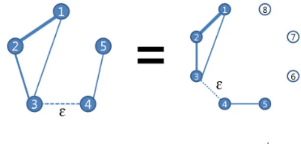
5.3 Manipulating the form of matrix; Chaining the disconnected networks with
Due to the application of markov chain rule, entropy rate of a random walk is not applicable if there are more than a graph.
However, in our case, the network of sharing vulnerabilities is split into several clusters because same vulnerabilities are discovered from the homogenous end devices. For example, the web servers using Apache 1.1 or Apache 1.3 can have same vulnerabilities, but IIS web servers do not share with Apaches. In order to join the two disconnected network, we connect the disconnected networks with , which is a very small value enough to be ignored at mathematical operation. Below ′ is the manipulated to connect the split networks; {1, 2, 3} and {4, 5}.
′
However, practically, we don't need to place on the virtual link between two split sub-networks. According to the formula (2), entropy rate is the summation of the terms, which is uncertainty to visit a next node. Mathmatically, the summation
keeps working even though the term is zero, which means that a certain node i does not have any relation with others like node 6, 7, 8. The zero term does not give any impact on the entropy rate. Therefore, putting is theoractically meaningful, but not really. Thus, the entropy rate of
and ′ is equal.
Fig. 4. Comparison of entropy rates between a network(, left) having two disconnected sub networks and a network(′, right) having two disconnected sub networks be chained with
5.4 Normalisation; Dividing entropy rate by maximum entropy rate
5.4.1 Invariant entropy rate
Before examining the invariance, which is a characteristic of entropy rate, let's arrange terms. Figure 5 is embodied from
. It shows the related nodes and the unrelated.
Fig. 5. Related nodes and unrelated in
-Related node : This node gets a positive reaction from the experiment by forming a
network or staying alone. In Figure 5, node 1,2,3,4,5 is related nodes. In this paper, these nodes have at least one vulnerability.
-Unrelated node : This node gets a negative reaction from the experiment, and node 6,7,8 are in this state. They are a vulnerability-free end devices in this experiment.
Let's assume there is another network
′, which is a modified from . The only difference is that ′ is the network connecting the two split sub-networks in
by . According to the above theorem, node 1,2,3,4,5 are related nodes from ′
and node 6,7,8 are unrelated nodes. ′ is composed of the related nodes in ′. Entropy rate is a kind of an invariant value in that it does not take care about the unrelated node. For example, against the different size of two networks, ′, ′, the entropy rate is same because entropy rate depends on (a) weight on connections, (b) the number of connections and (c) the structure of network. Since ′ and ′
have same weight on connections, same number of connections and same structure of network, the entropy rate is equal.
Fig. 6. Equality in entropy rate of ′(left) and ′(right)
5.4.2 Normalisation
In the previous, we have talked entropy rate is an invariant measure so that it
Fig. 7. Example of numerator (′,left) and denominator (
,right) in ERI
does not take care about the size of network. What we want to measure is the risk that an individual person might be faced with in a certain macro environment.
That's why we normalise the entropy rate of a -sized of network by dividing it with the maximum entropy rate of a -sized complete network. Also, this normalization brings back the impact of unrelated nodes shown at formula (4). The formula of ERI is shown at below.
(4)
Figure 7 is the example to show the proper parameters in calculating ERI. ′, which is left on the figure, is the network based on the observed data.
, which is on the right in the figure, is the complete network for a 8 number of nodes.
It will play a role to normalise ′ more precisely by bringing back the impact on node 6,7,8.
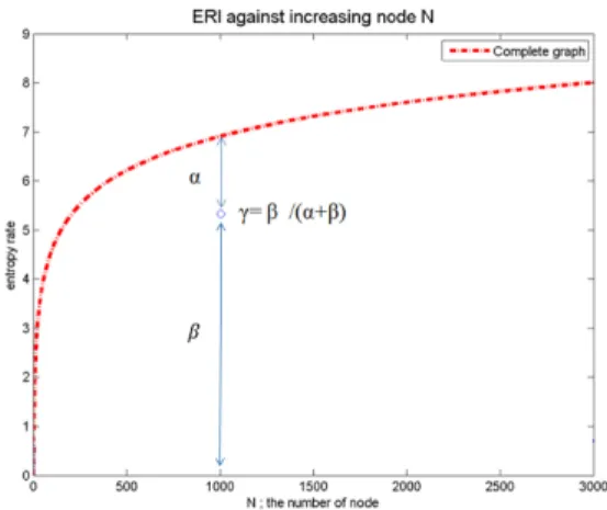
Firgure 8 shows the concept of ERI. The mechanism is as follows; Against the size of network, let's put as maximum entropy rate of a -sized complete network minus the entropy rate of the -sized network, and as the entropy rate of the
-sized network. is divided by , which is named as ERI. Due to the proportional characteristic, ERI stays
always between 0 and 1. Therefore, it is applicable to compare the different size of networks on an identical level.
Fig. 8. Entropy rate identifier (ERI) with entropy rates of sparse networks and complete networks
VI. Experimental Results
6.1.1 End devices' network;
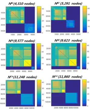
Figure 9 represents the networks of end devices(web servers) in Korea, Japan and China. All of six networks have two split sub-networks. The networks(, ,
) in the first column are the result of consecutive bipartite projections. ′, ′,
′ in second column are the result of connecting the unrelated nodes, which are vulnerability-free servers. It is distinct that has lots of unrelated nodes, which implies that Korea is sharing less vulnerabilities than other two countries.
Each country's networks tend to preserve their characteristics regardless of bringing the unrelated nodes. Both and ′
have a huge network and a tiny network, which means the network of web-servers in Japan is close in a form of a complete network. The networks of Korea(, ′) and China(, ′) are sparser than the
network of Japan(, ′). In the light of this fact, we can expect that Korea and China tend to less share vulnerabilities than Japan. Thus, they are more safe.
Fig. 9. Comparison of matrices of Korea, Japan, and China
6.1.2 Risk of end devices(web server) in Korea, Japan and China
Figure 10 shows the entropy rates of
′, ′ and ′ and their ERI. To tell the conclusion first, web servers in Japan are most exposed to threat and then in China and in Korea since ERI for three countries is in the order of ′(0.982948),
′(0.918286), ′(0.91615). We found the entropy rate of ′ is close with the maximum(1). In other words, ′ is in a form of complete graph whose all edges have a similar weight. From here, we can draw two points. First, servers in Japan are exposed on threats almost equally.
Second, almost all of the servers in Japan
are sharing at least a vulnerability between each other.
ERI support to decide more dangerous region in the view of sharing of vulnerabilities. It is not easy to judge which country is facing more risk between Korea and China on Fig9. For example, while ′ has two clearly different size of networks, but many virus-free servers, ′
has two balanced networks, but relatively much less number of virus-free servers than the its size. ERI solves this problem.
Even though there is no significant difference between two ERI (ERIKr:0.91615, ERICn: 0.918286), China has slightly higher ERI than Korea. Therefore, we can clearly make a decision that the servers in Japan are most sharing vulnerabilities and then in China and in Korea among the three countries in East asia.
Fig. 10. ERI against Korea, Japan, China
VII. Discussion
7.1.1 Application of ERI
We have talked about the network produced via forward projection, which makes it possible to compare the end devices' network for different countries. If we conduct consecutive bipartite
projections in a backward direction, we can make different meaning of network such as the networks between vulnerabilities, or threats. Also, depending on where you give a classification as if we have separated servers into a country level, you can construct more various networks. We will expand the application of ERI in next research. With this, we will find which threat is more popular in real, or which vulnerability is more risky due to the rampancy in our society.
7.1.2 Risk=ERI?
With ERI, it might be possible to measure the risk of a network. In order to measure the risk for a macroscopic environment, we applies ERI into the traditional risk formula; the combination of the likelihood of adverse event and the expected asset loss. We consider the likelihood of an event as the degree of sharing of vulnerabilities since the high sharing of vulnerabilities is likely to cause an incident. ERI represents the degree of sharing of vulnerabilities in a network.
Therefore, if we replace the score of fatality in CVSS to the expected damege term and multiply with ERI, the risk formula will be more sophisticate.
× (5)
where replaces likelihood of an event and
does expected asset loss in original formula.
7.1.3 Limitation
As ERI aims at calculating the risk of a huge group in numeric value in a short time, it is not appropriate to evaluate the risk of a specific system in accuracy where typical method takes all risk relative with
asset into account, for example, communication medium between devices such as router, switch, server, firewall, etc. Also, if the asset is customized product or unrecorded on CPE, the asset cannot be evaluated by ERI as we cannot retrieve any vulnerability information at CVE.
VIII. Conclusion
Until now, security risk analysis has been conducted in an organization. It requires to evaluate all connected network equipments in system to reflect all of the potential risk. However, in the era of IoE, it is more efficient to calculate only the end device, not considering the network equipment. In this paper, we present the risk analysis method to more focus on the relationship between end devices by using entropy rate. However, there were two problems to use the entropy rate as a measurement. In the case of the irreducible problem, we could avoid it theoretically by chaining disconnected sub-networks(or node) by . However, we found there is no difference between the entropy rates of a network having split networks and a network chaining those split networks by
. Also, by dividing an entropy rate with the maximum entropy rate, we can compare the entropy rates in different sized networks. According to the experiment measuring the average threat per a web server in East Asia by using proposed approach, servers in Japan are most sharing vulnerabilities and then in China and in Korea.
References
[1] Peltier and Thomas R, Information security risk analysis, 2nd Ed., CRC press, Taylor
& Francis Group 6000, Broken Sound
<저 자 소 개 >
김 광 원 (Kwangwon Kim) 학생회원
2010년 8월: University of Newcastle, IT학과 졸업 2011년 3월: 고려대학교 정보보호대학원 석사
<관심분야> 정보보호
윤 지 원 (Ji Won Yoon) 종신회원 2003년 2월: 성균관 대학교 정보공학 졸업
2005년 2월: University of Edinburgh, 정보학과 석사 졸업 2008년 11월: University of Cambridge 전자공학과 박사 졸업
2008년 2월~2009년 5월: University of Oxford, 로봇연구소 박사후과정 2011년 7월~2012년 8월: IBM 연구소 정규 연구원
2012년 9월~현재: 고려대학교 정보보호대학원 조교수
<관심분야> 신호정보처리, 응용통계, 도감청 탐지기술 Parkway NW, Suite 300 Boca Raton, FL
33487-2742, pp. 77-80, 2005.
[2] Cavusoglu, Huseyin, Birendra Mishra, and Srinivasan Raghunathan, “A model for evaluating IT security investments,”
Communications of the ACM, vol. 47, no. 7, pp. 87-92, Jul. 2004.
[3] Joh, HyunChul, and Y.K. Malaiya,
“Defining and assessing quantitative security risk measures using vulnerability lifecycle and cvss metrics,” SAM'11, pp. 10-16, Jul. 2011 [4] Stoneburner, Gary, A.Y. Goguen, and
Alexis Feringa, “Sp 800-30. risk management guide for information technology systems,” NIST, Jul. 2002 [5] Karabacak, Bilge, and Ibrahim
Sogukpinar, “ISRAM: information security risk analysis method,”
Computers & Security, vol. 24, no. 2, pp. 147-159, Mar. 2005
[6] Mell, Peter, Karen Scarfone, and Sasha Romanosky, “Common vulnerability scoring system,” Security & Privacy, vol.
4, no. 6, pp. 85-89, Nov. 2006
[7] Kotenko, Igor, and Mikhail Stepashkin.
"Attack graph based evaluation of network security." Communications and Multimedia Security. Springer Berlin Heidelberg, Jan. 2006.
[8] Phillips, Cynthia, and L.P. Swiler, “A graph-based system for network vulnerability analysis,” Proceedings of the 1998 workshop on New security paradigms, ACM, pp. 71-79, Sep. 1998.
[9] L.P. Swiler, Cynthia Phillips, and Timothy Gaylor, “A graph-based network-vulnerability analysis system,”
Sandia National Labs, Jan. 1998.
[10] Singhal, Anoop, and Xinming Ou,
“Security risk analysis of enterprise networks using probabilistic attack graphs,” NIST, Aug. 2011.
[11] Wang, Lingyu, Anoop Singhal, and Sushil Jajodia, “Measuring the overall security of network configurations using attack graphs,” Data and Applications Security XXI, Springer, pp. 98-112, Jul. 2007
[12] NVD: Common Vulnerability and Exposure (CVE), http://cve.mitre.org/about/index.html [13] Shodan:Shodan http://www.shodanhq.com/help