Transoceanic Propagation of 2011 East Japan Earthquake Tsunami

Article

http://dx.doi.org/10.4217/OPR.2014.36.3.225 September 2014

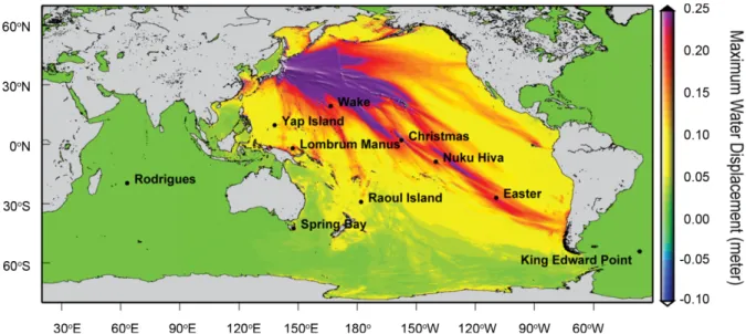
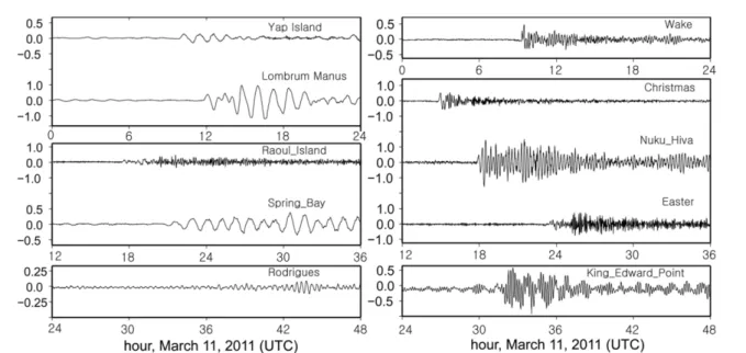
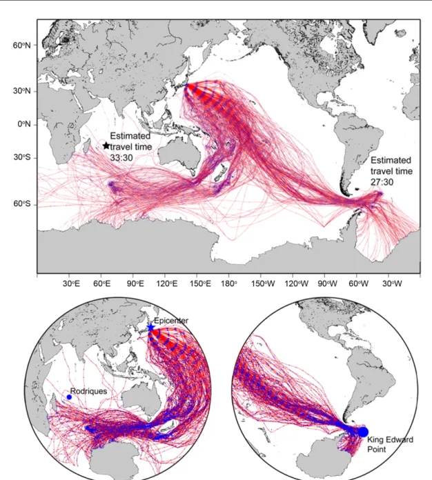
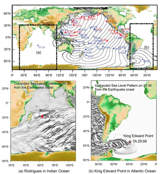
Transoceanic Propagation of 2011 East Japan Earthquake Tsunami

Byung Ho Choi

, Kyeong Ok Kim

, Byung Il Min

, and Efim Pelinovsky

1

Department of Civil and Environmental Engineering, College of Engineering, Sungkyunkwan University Suwon 440-746, Korea

2

Marine Radionuclide Research Center, KIOST Ansan 426-744, Korea

3

Nuclear Environment Safety Research Division, KAERI Daejeon 305-353, Korea

4

Department of Nonlinear Geophysical Processes, Institute of Applied Physics Russian Academy of Sciences, Nizhny Novgorod, 603950, Russia

5

Department of Applied Mathematics, Nizhny Novgorod State Technical University n.a. R.E. Alekseev Nizhny Novgorod, 603950, Russia

Abstract : The 2011 Tohoku earthquake triggered extremely destructive tsunami waves which propa- gated over the Pacific Ocean, Atlantic Ocean through Drake Passage and Indian Ocean respectively. A total of 10 tide-gauge records collected from the UNESCO/IOC site were analyzed through a band-pass digital filtering device to examine the observed tsunami characteristics. The ray tracing method and finite-difference model with GEBCO 30 arc second bathymetry were also applied to compare the travel times of the Tohoku-originated tsunami, particularly at Rodrigues in the Indian Ocean and King Edward Point in the Atlantic Ocean with observation-based estimates. At both locations the finite-difference model produced the shortest arrival times, while the ray method produced the longest arrival times. Val- ues of the travel time difference however appear to be within tolerable ranges, considering the propagation distance of the tsunami waves. The observed tsunami at Rodrigues, Mauritius in the west of the Mad- agascar was found to take a clockwise travel path around Australia and New Zealand, while the observed tsunami at King Edward Point in the southern Atlantic Ocean was found to traverse the Pacific Ocean and then passed into the Atlantic Ocean through the Drake Strait. The formation of icebergs captured by sat- ellite images in Sulzberger in the Antarctica also supports the long-range propagation of the Tohoku-orig- inated tsunami.

Key words : tsunami, 2011 Tohoku earthquake, tide-gauge records, numerical simulation

1. Introduction

The 2011 Tohoku earthquake, recorded to be 9.0 in magnitude, came about as a result of an undersea mega- scale thrust off the Pacific coast of Japan at 05:46 UTC (14:46 JST) on 11 March 2011. The earthquake is reported to be the fourth largest since the Chilean earthquake in 1960. The epicenter of the earthquake was between the Pacific and North American tectonic plates. The earthquake

triggered extremely powerful tsunami waves with a maximum run-up height of about 37.9 m that hit the Japanese Pacific-side coast minutes after the quake, in some cases inundating up to 10 km inland. Tsunami waves with smaller heights reached many other countries after several hours, affecting at least 20 countries, including most Asian countries in the western Pacific region, Australia and the entire Pacific coast of the American continent.

There are many researches on the 2011 Tohoku tsunami using numerical models (e.g., Chen et al. 2014; Choi et al.

*Corresponding author. E-mail : [email protected]

run-up heights. The propagations of tsunami waves to the North Pacific were also compared with wave heights and phases observed by DART buoys but the trans-oceanic propagation was not dealt with as an important subject.

Two other works, though not concerned specifically with the 2011 Tohoku tsunami, are worthy of mention. Liu et al. (1995) simulated the transoceanic propagation of the 1960 Chilean tsunami and the associated inundation at Hilo, Hawaii. Choi et al. (2003) estimated the trans- oceanic tsunami propagation from the Indian Ocean to the Atlantic and Pacific Oceans due to the 1983 Krakatau volcanic eruption using a numerical simulation.

The main goal of this paper is to analyze the tide-gauge records of the 2011 East Japan Pacific Coast-side Earthquake Tsunami in Atlantic and Indian Oceans. These collected data were filtered to remove the tidal components and were used to determine the observed tsunami characteristics (positive and negative amplitudes, heights, travel time). The analyzed results were also compared with the results of the ray tracing method and finite- difference model for the tsunami wave propagation in the framework of the linear shallow-water theory with the GEBCO 30 arc second bathymetry (www.gebco.net).

reduce noises. Tides were then removed by a high pass filter of 3dB cutoff for 60 minutes (Okada 1995; Baptista et al. 1992). The Butterworth filter, often termed a maximally flat magnitude filter, is a type of signal processing filter designed to obtain as flat a frequency response as is possible in the targeted frequency band. We are using the Butter worth filter function (function name is ‘butter’) of the well-known mathematical program MATLAB (ver.

2011a).

Fig. 1 displays the locations of tide-gauge stations selected in the study for the analysis of tsunami wave arrival times, which are for convenience superimposed on the distribution map of maximum tsunami wave heights computed using the finite-difference model described in Section 3. The selection of the tide-gauge stations was made on the basis of the computed propagation directions of the Tohoku-originated tsunami wave. We can see from the underlying map that the main axis of the tsunami propagation was aligned southeastward with several sub- axes. It is noted that except for the northwestern Pacific region off Japan the maximum wave heights in Pacific region are relatively small. Our concern in this study is, however, directed to the long-range propagation process

Fig. 1. Locations of selected tide gauge stations for the tsunami arrival analysis superimposed on the maximum water

displacement map of 2011 Tohoku-originated tsunami waves computed using a finite-difference model

so that the sites located in the Southern Pacific were mostly chosen along with two additional points, one in the Indian Ocean and the other in the Southwestern corner of the Atlantic Ocean.

We first examined the time series of the filtered sea level variations (Fig. 2). While the propagation of tsunami waves from the east side of Japan to the Atlantic Ocean and Indian Ocean is hard to confirm from Fig. 1, very distinctive tsunami waves are visible on all tide-gauge records including King Edward Point in the Atlantic Ocean, and Rodrigues in the Indian Ocean. The arrival time of tsunami waves can be visibly determined in all records in the South Pacific but not at King Edward Point

and Rodrigues. Difficulty in estimating the arrival time from the time series records at stations located far away from the epicenter is expected because the tsunami waves experience significant amount of topographic modification and wave dispersion in the course of propagation, resulting in time-varying sea surface elevation with different periodicities. The starting time when a series of displacements with significant heights occurs is, though subjective to a certain degree, considered as the tsunami arrival time.

According to our evaluation, the tsunami wave arrived at King Edward Pointat 07:44 UTC on 12 March (travel time of about 26 hours) with a wave height of 76 cm, while it arrived at Rodrigues at 12:58 UTC on 12 March Fig. 2. Tsunami records of UNESCO/IOC for the 2011 Tohoku earthquake tsunami. Note the difference in scales and

x-axis of time

Table 1. Tsunami travel times and maximal tsunami wave heights evaluated from tidal records

Points Location

(Lon, Lat)

Tsunami travel time (HH:MM)

Positive amplitude (m)

Negative amplitude (m)

Height (m)

Wake 166.62 W 19.29 N 03:31 0.480 0.336 0.816

Yap Island 138.12 W 9.51 N 04:11 0.213 0.207 0.420

Lombrum Manus 147.37 W 2.04 S 06:01 1.051 1.319 2.370

Christmas 157.47 E 1.98 N 09:00 0.580 0.545 1.125

Raoul Island 177.89 E 29.28 S 11:52 0.295 0.230 0.525

NukuHiva 140.08 E 8.91 S 12:04 1.509 1.569 3.078

Spring Bay 147.93 W 42.55 S 15:33 0.373 0.348 0.721

Easter 109.45 E 27.15 S 17:53 0.762 0.721 1.483

King Edward Point* 36.50 E 54.28 S 25:58 0.357 0.403 0.760

Rodrigues** 63.42 W 19.68 S 31:12 0.184 0.117 0.301

N.B. **Atlantic Ocean

N.B. **Indian Ocean

Fig. 3. Computed spectra of filtered tsunami oscillations at tide gauge records of Rodrigues and King Edward Point.

Periods of the main spectral peaks are indicated

Fig. 4. Frequency-time plots (f-t diagrams) for tide gauge records (station names in plot)

(travel time of about 31 hours) with a wave height of 30cm. Full details of the travel times and wave heights are summarized in Table 1. It is evident that the tsunami wave height is the largest at Nuke Hiva.

To examine the frequency characteristics the filtered data sets were processed by FFT (Fast Fourier Transform) spectrum and Wavelet analysis. Fig. 3 shows the FFT spectrum at two locations, Rodrigues and King Edward Point. The spectra show that for Rodrigues the energy is focused in a 24 minute period, while for King Edward Point energies are focused in two periods, namely 1 hour and 12 minutes. It is likely that, since the path of wave propagation to King Edward Point is topographically simpler than that to Rodrigues and the wave energy dissipation rate in the course of propagation is therefore lower, the tsunami waves recorded at King Edward Point have shorter periods than Rodrigues. Fig. 4 shows the arrival times determined using the Wavelet analysis. The vertical dashed line labeled “E” denotes the time of earthquake occurrence and the black vertical line labeled

“TA” denotes the time of tsunami wave arrival. Again, all results except for King Edward Point and Rodrigues clearly show the arrival times. Since the arrival times in King Edward Point and Rodrigues were difficult to determine, numerical calculations are additionally carried out in the next section.

3. Numerical Calculations of the Tsunami Travel Time

Calculation of the tsunami travel time for the tide- gauge locations is performed in the framework of the ray tracing method (Choi et al. 2003). Ray tracing equations are:

(1)

(2) Where t is time, θ and ϕ are the latitude and longitude of the ray, respectively, is the inverse of long-period wave speed, g is the gravity acceleration, h( θ, ϕ) is the water depth, R is the radius of the earth, and ζ is the ray direction measured counter-clockwise from the South. Details of the numerical integration are given in Choi et al. (2003). The model assumes that the wave length is larger than the local ocean depth but smaller than the large-scale variation of bottom topography. The code (Choi et al. 2003) calculates the first wave arrivals only.

Pelinovsky et al. (2005) fully discussed the comparison of a range of ray methods along with the methodology of tsunami analysis with a numerical filter. The limitation of the ray tracing method is discussed in the paper by Satake (1988).

The location of the source in the numerical simulations was arranged to be close to that of the 2011 Tohoku Tsunami as much as possible. A total of 7,200,000 rays were used and initially distributed uniformly. For the correct calculation of the travel time some additional rays were used. The bathymetry was taken from the 30-sec GEBCO dataset. Computed results of tsunami travel times are shown in Fig. 5, which are generally in reasonably good agreement with observed times in the Pacific Ocean.

It is confirmed that tsunami waves initially affected the western basin of the Pacific Ocean, and are separated into two branches, one branch turning around Australia and New Zealand in a clockwise direction passing into the Indian Ocean and another branch heading for the Drake Strait passing into the Atlantic Ocean with reduced energy. It is noted that use of the ray tracing method produces the tsunami travel time of about 33.5 hours to Rodrigues (that is, a late arrival by about 2.3 hours when observations are compared), while the travel time was 27.5 hours to King Edward Point (that is, a late arrival by about 1.5 hours when observations are compared).

Difficulty in determining the correct arrival time on the basis of the filtered data has already been commented on in the section 2, because it is hard to judge whether observed disturbances are real tsunami waves or not. The ray model has a limitation in finding the path of the first reached tsunami wave because the estimated travel time is dependent on the number of rays used.

The finite-difference model (Choi et al. 2003) is constructed to simulate the tsunami generation and propagation using the linear shallow-water equation with a spherical coordinate system. The basic equations are

(3) In the equations above, P and Q are discharges per unit width in the meridional and zonal directions, respectively, R is radius of the earth, and f is the Coriolis parameter.

The model has a high horizontal grid resolution of 30 sec θ

d t --- d cos ξ

---, ϕ nR d t

--- d sin ξ Rsin θ ---

= =

ξ d

t --- d sin ξ

n

R ---∂ n

∂θ --- cos ξ n

Rsin θ --- ∂ n

∂ϕ --- sin ξsinθ --- nR –

+

=

n = ( ) gh

∂η ∂t --- 1

Rcos φ --- ∂ P

∂χ --- ∂

∂φ --- Qcos ( φ ) +

+ = 0

∂P ∂t --- gh

Rcos φ ---∂η

--- fQ ∂χ –

+ = 0

∂Q ∂t --- gh

---∂η R --- fP ∂φ –

+ = 0

(approximately 750 m in mid-latitude area). Integration was carried out with a time step of 0.5 sec. The land boundary conditions are given by the no-flux condition, and the radiation boundary scheme is employed along the north open boundary. The south boundary is closed by the Antarctica and other horizontal boundaries are treated through a cyclic boundary scheme. The initial surface water displacement is computed using 39 tele-seismic broadband P waveforms, 22 broadband SH waveforms, and 55 long-period surface waves and azimuthal distribution.

Waveforms are converted to displacement by removing the

instrument response and then used to constrain the slip history based on a finite fault inverse algorithm (Heyes 2011).

Fig. 6 shows the snapshots of the Tohoku-originated tsunami propagation pattern every 3 hours computed using the finite-difference model. The full animation can be seen in http://sites.google.com/site/bhchoiskku/trans- oceanic. Fig. 7 (upper) shows the hourly isochrones of the tsunami travel time from the source area computed using the finite-difference model and the positions of UNESCO/

IOC tide gauges around the Pacific Ocean together with Fig. 5. Red lines indicate the Tsunami ray path from epicenter to Rodriques and King Edward Point. Blue dots indi-

cate the hourly reached positions

the travel times deduced from the observation data for comparison. It is noted that the computed travel times are in agreement with observation-based travel times with reasonable accuracy. Fig. 7 (lower) are the spatial distributions

computed using the finite-difference model in regions marked in dashed lines around Rodrigues and King Edward Point 29.5 and 24.5 hours after the onset of the Tohoku earthquake, respectively. The tsunami travel times Fig. 6. Snapshots of water surface elevation over Pacific Ocean every 3 hours due to 2011 Tohoku Great Earthquake

Tsunami

to Rodrigues and King Edward Point computed using the numerical model is shorter than those computed using the

ray tracing method and also deduced from the observations.

Table 2 summarizes the detailed comparison results obtained from the ray tracing method, the numerical model and the observations.

Impacts of tsunami waves are known to often break off icebergs at a faraway distance. After the occurrence of the Tohoku-originated tsunami the satellite images showing the process of creating icebergs in Sulzberger in Antarctica were captured by the European Space Agency/Envisat.

Fig. 8 shows the location of Sulzberger and the sequential calving images, supporting the arrival of tsunami waves of 2011 Tohoku origin.

Fig. 7. Upper) Hourly isochrones of the tsunami travel time from the source are drawn in solid thin lines. The posi- tions of UNESCO/IOC tide gauges in Pacific Ocean are marked with values of tsunami arrival time. Lower) Spatial distributions of sea surface displacement are shown in regions marked by dashed line in upper figure:

(a) Rodrigues after 29.5 hours, (b) King Edward Point after 24.5 hours since the onset of Earthquake

Table 2. Tsunami travel times deduced from observation and the application of the ray tracing and finite- difference numerical models at King Edward Point and Rodrigues with time difference com- paring with observations

King Edward Point Rodrigues

Observation (Table 1) 25:58 31:12

Ray tracing method 27:30 (+1.5 hr) 33:30 (+2.3 hr)

Numerical model 24:30 (-1.5 hr) 29:30 (-1.7 hr)

4. Conclusion

The 2011 East Japan Pacific Coast-side Earthquake Tsunami was propagated on a transoceanic scale and the water displacement caused by the tsunami wave was detected in many worldwide tide-gauge records. The tsunami wave even created icebergs as observed by satellite images in Antarctica. The tide-gauge records containing the signal of the Tohoku-originated tsunami waves were analyzed to examine the observed tsunami characteristics in the Pacific Ocean, Indian Ocean and near the southwestern corner of the Atlantic Ocean.

Analysis shows that tidal-gauge records in the Pacific Ocean established accurate estimates of the arrival time, while analysis of two tidal-gauge records in the Indian Ocean (Rodrigues) and Atlantic Ocean near the Drake Passage (King Edward Point) revealed the difficulty of making correct estimates of the arrival time. This may be attributed to the presence of a significant amount of tidal noises within and near the filtered frequency bands.

Attempts to use the ray tracing method and finite- difference model with detailed 30 arc second bathymetry were made to compare the arrival times with regard to the Indian and Atlantic Oceans. The arrival times computed from the wave ray-based refraction diagram and numerical simulation using the linear shallow water equation are generally in reasonable agreement with observation-based estimates in the Pacific Ocean. The three approaches however produced noticeable differences in the results at Rodrigues in the Indian Ocean and King Edward Point in the Atlantic Ocean. Comparing both locations with the observation-based estimates, the finite-difference model

produced shorter arrival times, while the ray method produced longer arrival times. Values of the travel time difference however appear to be within tolerable ranges, considering the distance of the propagation of the tsunami waves.

Although the simulations are useful in providing information on the path of the tsunami wave propagation and the travel times, refinement of the model resolution with use of better information on bathymetry is however needed to reproduce wave heights accurately. Investigation on the long-distance propagation of tsunami waves using more sophisticated nonlinear models, for example, the model described by Yoon et al. (2007), are of course required for future study.

Acknowledgements

This study was supported by the China-Korea cooperative research project funded by CKJORC as well as a major project titled the development of the marine environmental impact prediction system funded by KIOST. EP thanks State Contract No.2014/133.

References

Baptista MA, Miranda P, Victor LM (1992) Maixmum entropy analysis of Portuguese tsunami data the tsunamis of 28.02.1969 and 26.05.1975. Sci Tsunami Hazards 10(1):9-20

Chen C, Lai Z, Beardsley RC, Sasaki J, Lin J, Lin H, Ji R, Sun Y (2014) The March 11, 2011 Tōhoku M9.0 earthquake-induced tsunami and coastal inundation along Fig. 8. Location of Sulzberger and the sequential images of Sulzberger Ice Shelf breaking (Credit: NASA/Goddard,

http://www.nasa.gov/topics/earth/features/tsunami-bergs.html)

Runup Heights of the 2011 off the Pacific Coast of Tohoku Earthquake Tsunami Based on Numerical Simulations. Open Oceanogr J 6:5-13

Heyes G (2011) Finite Fault Model, Updated Result of the Mar 11, 2011Mw 9.0 Earthquake Offshore Honshu, Japan;

2011. http://earthquake.usgs.gov/earthquakes/eqinthenews/

2011/usc0001xgp/finite_fault.php Accessed 1 Sep 2014 Kim KO, Choi BH, Pelinovsky E, Jung KT (2013) Three-

dimensional simulation of 2011 East Japan-off Pacific coast earthquake tsunami induced vortex flows in the Oarai port. J Coastal Res SI65:284-289

Liu PLF, Cho YS, Yoon SB, Seo SN (1995) Numerical Simulations of the 1960 Chilean Tsunami Propagation and Inundation at Hilo, Hawaii. Adv Nat Technol Haz 4:99-115

Sasaki J, Ito K, Kazunori I, Suzuki T, Wiyono RUA, Oda Y, Takayama Y, Yokota K, Furata A, Takagi H (2012) Behavior of the 2011 Tohoku earthquake tsunami and resultant damage in Tokyo Bay. Coast Eng J 54(1):

1250012

Satake K (1988) Effects of bathymetry on tsunami propagation:

application of ray tracing to tsunamis. Pure Appl Geophys 126:27-36

Yoon SB, Lim CH, Choi J (2007) Dispersion-correction finite difference model for simulation of transoceanic tsunamis. Terr Atmos Ocean Sci 18(1):31-53

Received Aug. 27, 2014

Revised Sep. 8, 2014

Accepted Sep. 15, 2014