The Relationship between Default Risk and Asset Pricing: Empirical Evidence from Pakistan

Print ISSN: 2288-4637 / Online ISSN 2288-4645 doi:10.13106/jafeb.2021.vol8.no3.0717

The Relationship between Default Risk and Asset Pricing:

Empirical Evidence from Pakistan

Usama Ehsan KHAN

, Javed IQBAL

Received: November 30, 2020 Revised: February 01, 2021 Accepted: February 16, 2021

Abstract

This paper examines the efficacy of the default risk factor in an emerging market context using the Fama-French five-factor model. Our aim is to test whether the Fama-French five-factor model augmented with a default risk factor improves the predictability of returns of portfolios sorted on the firm’s characteristics as well as on industry. The default risk factor is constructed by estimating the probability of default using a hybrid version of dynamic panel probit and artificial neural network (ANN) to proxy default risk. This study also provides evidence on the temporal stability of risk premiums obtained using the Fama-MacBeth approach. Using a sample of 3,806 firm-year observations on non-financial listed companies of Pakistan over 2006–2015 we found that the augmented model performed better when tested across size-investment-default sorted portfolios. The investment factor contains some default-related information, but default risk is independently priced and bears a significantly positive risk premium. The risk premiums are also found temporally stable over the full sample and more recent sample period 2010–2015 as evidence by the Fama-MacBeth regressions. The finding suggests that the default risk factor is not a useless factor and due to mispricing, default risk anomaly prevails in the Pakistani equity market.

Keywords: Asset Pricing, Default Risk, Fama-French Five-Factor Model, Emerging Market JEL Classification Code: G11, G12, G32, G33

Several studies have been conducted on whether the default risk is related to the cross-section of equity returns and if it is accurately priced. However, the results are often conflicting. For instance, Chan and Chen (1991) argue that the size premium captures the default risk as a distressed firm’s stock loses its market value and fall into the small-stock portfolio. In addition, Chen and Zhang (1998) show that firms with high book-to-market have low earnings along with high leverage that translates higher default risk. Similarly, Fama and French (1996) contend that high returns to distressed stocks are due to their near bankruptcy, and there is a default risk premium that drives high returns and factors i.e., high-minus- low (HML) and small-minus-big (SMB) capture default risk. They maintain the position that weak firms with persistently low earnings have high book-to-market value and positive slopes on high-minus-low (HML), similarly, small firms generally have low access to external finance and volatile cash flows, therefore, such firms are more likely to default which implies the significance of SMB factor in proxying default risk. These studies postulate the “distress hypothesis” by explaining the size and value effect, that is, distressed firms earn higher returns due to the high loadings on size and value factor as compared to

1

First Author and Corresponding Author. Ph.D. Candidate, Applied Economics Research Centre, University of Karachi, Karachi, Pakistan [Postal Address: R-220 Sector 15-A/1, Bufferzone, Karachi, Pakistan] Email: usama.ehsan@gmail.com

2

Associate Professor, Institute of Business Administration, Karachi, Pakistan. Email: javed_uniku@yahoo.com

© Copyright: The Author(s)

This is an Open Access article distributed under the terms of the Creative Commons Attribution Non-Commercial License (https://creativecommons.org/licenses/by-nc/4.0/) which permits unrestricted non-commercial use, distribution, and reproduction in any medium, provided the original work is properly cited.

1. Introduction

A firm defaults when it fails to fulfill its monetary

obligation. Stakeholders measure default risk by the financial

condition of the firm and induce the lenders to require

premium from borrowers. This premium is a decreasing

(increasing) function of financial soundness (vulnerability)

of the firm. The effects of default risk on equities are

more subtle than on corporate debt. Stocks of financially

distressed firms possess higher risk but deliver anomalously

low returns as stocks of financially distressed stocks tend

to move together and their risk cannot be diversified away

(Campbell, Hilscher, & Szilagyi, 2008).

non-distressed firms (Bauer, 2012). Other studies such as Dichev (1998), Campbell et al. (2008), Vassalou and Xing (2004), Gharghori, Chan, and Faff (2007), however, take a contrary position that size and value risk factors contain some information related to default but inconsistent with the argument that these factors are compensation for default risk.

The modern financial theories such as the trade-off theory of Modigliani and Miller (1958) contend that shareholders perceive higher default risk with an increase in the debt component, therefore, require a higher expected return.

With imperfect capital markets and prevailing information asymmetries, Shleifer and Vishny (1997) argue that debt could be an efficient way to reduce agency costs. Therefore, an increase in leverage can influence the likelihood of default and subsequently high expected equity return which is in line with the trade-off theory. However, most of the empirical evidence suggests that higher default risk is unable to attract higher returns and distress risk-return anomaly continues to prevail (George & Hwang, 2010).

Fama and French (2015) suggest that their five-factor model is superior to the three-factor model. Therefore, rather than reconciling puzzling evidence, the current study examines whether these five factors proxy default risk or a separate individual role of the default risk factor is still inevitable in explaining cross-sectional variations in equity return. Moreover, as most of the studies are focused on developed countries, an out-of-sample examination is necessary before ensuring any conclusions as pointed out by Lo and MacKinlay (1990). Emerging markets such as Pakistan provides an ideal setting for the external validity of the Fama-French five-factor model in general and testing default risk factor in particular. Drobetz, Sturmer, and Zimmermann (2002) provide two justifications to constitute emerging markets a viable stand-alone asset class. First, higher economic growth drives higher expected returns in emerging markets. Second, investments in emerging markets provide a hedge against losses in more established markets due to their lack of global integration. However, emerging stock markets are exposed to several anomalies. Hoang, Phan, and Ta (2020) find evidence on prevailing nominal price anomaly in the Vietnamese equity market.

Similarly, Pojanavatee (2020) find liquidity in addition to market and value risk factors capable of explaining equity returns for Thailand’s Consumer Products. While considering trade frictions in Indonesia, Nurhayati and Endri (2020) observe that trading frictions enhance exposure to market risk with little impact on size and value factors in the context of the Fama-French three-factor model. In a recent study, Asis, Chari, and Haas (2020) document a positive distress risk premium in emerging market equities including Pakistan. It is also argued that global financial conditions are instrumental in explaining financial distress in emerging economies. Foye (2018) struggles to find the five-factor model useful for some Asian markets including China, India,

Indonesia, Malaysia, Philippines, South Korea, Taiwan, and Thailand.

Our motivation for testing the five-factor model augmented with the default risk factor in a Pakistani market runs deeper than just providing the out-of-sample test.

As compared to the sample used by Foye (2018), a low bankruptcy protection environment is evident in Pakistan as it is ranked lower on the Doing Business – World Bank Insolvency indicator (Doing Business, 2020). Moreover, the Pakistani equity market was categorized among best performing and worst performing by MSCI on multiple occasions, more recently, Asia’s best-performing stock market in 2016 and the worst one in 2017 when comparing PSX’s return with MSCI Emerging Markets Index. Political and macroeconomic uncertainties also make Pakistan a potential candidate, in particular, none of the democratic regimes in Pakistan has ever completed its tenure since Pakistan’s independence. Extreme volatilities due to all these facts could suppress empirical regularities and a lack of investor sophistication may make default risk not be adequately discounted in stock prices and default risk anomaly may hold in those markets.

Our chosen setting offers the following key merits. Firstly, we develop an asset pricing framework for the Pakistani market which is exposed to multifaceted risk exposures similar to other emerging markets that bear different risk-return characteristics in contrast to the developed economies. The current study employs the Fama and French (2015) five-factor asset pricing model and augments it with the default risk factor. We test the significance of the augmented five-factor model for different portfolios sorted on the firm’s financial characteristics as well as on industry. Secondly, we examine whether five factors of Fama-French proxy default risk. There exists some evidence for some of these factors proxying default risk. For instance, Fama and French (1996) contend that SMB and HML proxy default risk. There is also evidence that that investment factor inherent premium for default risk (Campbell et al., 2008).

Moreover, Griffin and Lemmon (2002) found that firms with a higher probability of default have weak current profitability, therefore, default risk may be captured by profitability factor.

We investigate whether the default risk factor is non-redundant in a five-factor asset pricing framework. Finally, to examine whether Fama-French five factors proxy default risk, this study constructs a default risk factor (DEF) as the difference between equity returns on firms with a high probability of default and that of the low probability of default. For this purpose, we estimate the probability of default using a competitive bankruptcy prediction model that combines features of traditional econometrics and data science models i.e., hybrid- ANN similar to Khan, Iqbal, and Iftikhar (2020). If the default risk is systematic then a significantly positive risk premium for the default risk factor exists.

The findings of the study can be summarized as follows.

Based on the full-period, i.e., 2005–2015, the analysis of

portfolio sorts on multiple characteristics, it is found that the default risk premium is positively significant, therefore, systematic. When splitting into two sub-periods, the second period (i.e., 2010–2015) witnesses statistically meaningful default risk premiums for most of the portfolio sorts.

However, the default factor premium loses its significance for industry portfolios for both full period and sub-periods. We also reject the notion that the default risk factor is ‘useless’

across all portfolio sorts as well as for industry portfolios.

The study also uncovers evidence that the investment factor contains some information related to default, however, none of the Fama-French captures default risk.

The rest of the study is organized as follows. Section 2 provides a review of the existing literature. Section 3 discusses the empirical framework. Section 4 describes the data employed for this study. Section 5 exhibits the result and, finally, section 6 concludes the study.

2. Literature Review

The theoretical finance posits that higher risk should be rewarded with a higher return, however, empirical studies show stocks of distressed firms earn anomalously lower returns than that of non-distressed firms. There exists mounting evidence that the relationship between default risk and equity returns is irrationally negative in some markets while significantly positive in other markets.

Dichev (1998) explains such a relationship due to the mispricing of default risk in equity returns. It brings evidence pertaining to the default risk-return relationship by using Ohlson’s (1980) and Altman’s (1968) bankruptcy risk measures for proxying default risk. It is found that there exists a negative relationship between default risk and equity returns inconsistent with economic rationale. Ghargori, Chan, and Faff (2009) also provide evidence that default risk is negatively related to returns and advocate that size and value factors are not proxying default risk. Their results suggest that the negative relationship between the probability of default and equity return is not due to volatility, leverage or momentum effects. Avramov and Zhou (2010) find the implications of financial distress for the profitability of anomaly-based strategies and claim that these strategies derive their profitability from taking short positions in high credit risk firms that experience credit deteriorating conditions.

Other studies present a statistically positive relationship between default risk and return concluding the systematic nature of default risk. For instance, Griffin and Lemmon (2002) use O-score to proxy distress risk and found that among the highest distressed firms, the difference in returns between high and low book-to-market (BM) stocks is more than twice than the other firms. Such a behavior is not explained by Fame-French three-factor model and is often linked to profitability and leverage. Vassalou and Xing

(2004) found that highly risky firms command a higher return only to the extent that they are small in size and have a high book-to-market ratio. However, their study concludes that default risk is systematic based on results from system analysis of the default-augmented pricing model. Chan, Faff, and Kofman (2011) suggest that the default factor does not explain the success of size and that the default indicator has a complementary role with small minus big (SMB) and high minus low (HML) factors. Agarwal and Taffler (2008), Gharghori et al. (2007) and Campbell et al. (2008) found similar results that the three Fama-French factors do not proxy default risk.

Fama and French (2016) claim that list of anomalies shrinks in the Fama-French five-factor model. However, default risk anomaly is not discussed. Other studies also do not formally test whether factors involved in the latest version of asset pricing, i.e., Fama and French’s (2015) five-factor model capture default risk. The asset-pricing literature on the existence of default risk is somewhat sparse and focuses mainly on developed markets. Developing countries, on the other hand, an inherent relatively high sovereign risk which is associated with an aggregate default risk of a country’s corporate sector (Altman & Rijken, 2011).

The equity market of Pakistan is relatively segmented and safer from international shocks offering immense potential for international diversification. In addition, relative to the market capitalization trading activity is high depicting the typical nature of the market (Iqbal, 2012). Pakistani stock market has also been ranked among the best performing market on multiple occasions e.g., in the last quarter of 2019. In general, emerging and frontier markets provide opportunities for alpha-seeking investors, therefore, the current study aims to provide insights into these unique characteristics.

3. Empirical Framework

3.1. Fama-French Five-Factor Model

The Fama and French (1993) three-factor model is designed to capture cross-sectional variations due to size (based on market capitalization) and price ratio, i.e., book- to-market in addition to the excess market return. The basic three-factor model can be written as:

r

= α

+ b

r

+ s

SMB

+ h

HML

+ e

(1)

In equation (1), r

is the excess return on i at time t over

risk-free rate of interest at time t, r

is the excess market

return over risk-free interest rate at time t, SMB

(small

minus big) is the difference between the diversified portfolio

returns of small stocks and big stocks, HML

is the return

on a diversified portfolio of high B/M minus the return of

diversified portfolio on low B/M and e

is the error term.

Extant literature evident widespread success of the three- factor model in explaining the cross-sectional variation of stock return in the USA and other countries. However, the theoretical rationale for factors has not been provided.

Fama and French (2015), therefore, provide theoretical justification based on the dividend discount model, and, at the same time introduce profitability and investment factors additionally to the three-factor model. The dividend discount model implies that the market value of a stock share is the discounted value of expected dividends per share. To test the Fama-French five-factor model, Fama and French (2015) run the regressions of excess portfolio return on excess market return, size, value, investment, and profitability risk factors.

We innovate the model by introducing a default risk factor additionally, the augmented Fama-French five-factor model takes the following form:

r b r s h c

r d e

it i i mt i t i t i t

i t i t it

 SMB HML CMA

RMW DEF (2)

In equation (2), r

is the excess return on portfolio i at time t over risk-free rate of interest at time t, r

is the excess market return over risk-free interest rate at time t, SMB

(small minus big) is the difference between the diversified portfolio returns of small stocks and big stocks, HML

is the return on a diversified portfolio of high B/M minus the return of diversified portfolio on low B/M, CMA

is the return on a portfolio of the stocks of the conservative (low) investment minus that of aggressive (high) investment stocks, RMW

is the difference of the returns on portfolios of stock with robust and weak profitability, and DEF

is the return on diversified portfolios returns of the stocks of a high probability of default minus to that of a low probability of default

. The respective factor risk exposures on the aforementioned factors are b

, s

, h

, c

, r

, and d

. If the model captures the cross-section of returns then the null hypothesis that all α

are jointly equal to zero cannot be rejected. Gibbons, Ross, and Shanken (1989) (GRS) propose F-test to test this hypothesis.

The current study employs Fama and MacBeth (1973) two-step regression for estimating risk exposures and subsequent risk premiums. The error terms obtained in cross- sectional regressions are almost certainly autocorrelated and heteroskedastic. To correct this problem, we employ Newey- West heteroskedasticity and autocorrelation corrected (HAC) standard errors to compute t-statistics.

3.2. Temporal Stability Diagnostic

In order to examine the temporal stability of the default risk factor in the non-financial sector of Pakistan’s equity market, we divide the time series into two sub-periods demarcated by 2009 such that the earlier period is from January 2006 to December 2009 and the latter period is

over January 2010 to December 2015. This sub-period classification may serve a better cut-off point for testing temporal stability because of the three reasons: (i) Global Financial crisis of 2008–09, although Pakistan is not directly a victim, however, global economic slowdown affected demand for the country’s exports and firms at hand are mostly export-oriented, (ii) political regime switch, an era of democratic revival has started in 2009, and (iii) major adverse shift in the textile industry (textile sector accounts for nearly 42 percent of the research’s sample).

3.3. Useless Factor Test

One potential issue is that the introduction of a new factor may misspecify the asset pricing model. Kan and Zhang (1999) show concern that, when a factor is not useful in time series, then t-statistics from Fama and MacBeth (1973) regressions can be biased. The intuition is that when a factor is useless, i.e., being independent of all the portfolio (or stock) return, the second-pass cross-sectional regression captures the factor risk of useless factors more often. We involve the useless factor test of Kan and Zhang (1999) to test whether a new factor has pervasive importance across the test assets.

We jointly test the null hypothesis H0: d

= d

= …. = d

= 0, where n is the number of portfolios. Rejection of the null hypothesis concludes that the default risk factor (DEF) is not useless. The test is extended over all three sets of sorted portfolios as well as industry portfolios.

4. Data and Methods 4.1. Dataset

The data consist of monthly adjusted closing prices of 346 non-financial listed stocks, as well as data on the Karachi Stock Exchange 100 index (KSE-100), which are taken from January 2006 to December 2015 from the Bloomberg database. Stocks are selected based on available time series over a given period for which the prices have been adjusted for dividends, stock split, merger, and corporate actions.

Market capitalization for each listed stock is not recorded on monthly basis, therefore, series of annual market capitalization along with other financial ratios are obtained from the State Bank of Pakistan’s publication Financial Statement Analysis of Companies (Non-Financial). The data on macroeconomic indicators are taken from Thomson Reuters Datastream.

4.2. Construction of Portfolios

The study employs mainly four sets of portfolios as

our test assets. Size, value, profitability, investment, and

default are proxied by market capitalization, the book to

market, operating profit ratio, growth in total assets, and the probability of default respectively. The probability of default is estimated hybrid-ANN, i.e., hybrid of dynamic panel probit and artificial neural network model as the model attains higher accuracy of classification as compared to other competing approaches for the non-financial sector of Pakistan

. Monthly value-weighted returns are calculated for all sets of portfolios and are portfolios are rebalanced at an annual frequency.

4.2.1. Size-B/M-Profitability-Investment-Default Sorted Portfolios

All stocks in the sample are independently ranked on size, book-to-market (BM), profitability (OP), investment (INV), and the probability of default (PD), and are allocated into two groups according to the median split. The intersection of two size, two book-to-market, two investment, two profitability and two PD groups formed 32 portfolios.

4.2.2. Size-Default and Investment-Default Sorted Portfolios

Two subsets of 16 value-weighted portfolios over the full sample period are constructed. Specifically, all stocks are independently sorted on size and probability of default and are then allocated into four groups based on quartile split. The intersection of four size and probability of default constitutes the first subset of 16 portfolios. The second subset of 16 portfolios is constructed in a similar manner but sorts are based on investment and probability of default.

4.2.3. Size-B/M-Default, Size-Profitability-Default and Size-Investment-Default Sorted Portfolios Three subsets of eight value-weighted portfolios are constructed. First, all stocks are independently sorted on size, book to market, and the probability of default based on the median split, upon an intersection, yielding the first set of eight portfolios. The other two subsets of portfolios are constructed using characteristics such as size, profitability, default; and size, investment, and default.

4.2.4. Industry Portfolios

The industry portfolios are formed by classifying all stocks in a sample into 16 industry subgroups based on the industry classification of the State Bank of Pakistan.

The use of stock characteristics to group portfolios in a particular way is subject to potential data snooping and measurement error bias (Lo & MacKinlay, 1990). For instance, Ang, Liu, and Schwarz (2010) emphasize that sorting stocks into portfolios by characteristics that are correlated with returns would affect risk premiums.

Industry portfolios allow circumventing potential issues

for data mining from the construction of portfolios. While these portfolios do not need to be balanced provides an advantage, Fama and French (1997) caution temporal instability of factor loadings which is tested in this study for industry portfolios as well as for portfolios sorted on firms’ characteristics.

4.3. Creation of Factors

To construct Fama and French’s five factors, we follow the first approach among the three adopted by Fama and French (2015). The value and size factors are based on independent sorts of stocks into three B/M groups and two size groups. The intersection of sorts produces six value- weighted portfolios. The size factor, SMB

, is the difference between the monthly average return of three small portfolios and that of three big portfolios. The value factor, HML, is the average return on two high B/M portfolios minus the average return on two low B/M portfolios.

The conservative minus aggressive (CMA) investment factor portfolios and robust minus weak (RMW) factor portfolios are constructed in a similar manner as the HML factor portfolios using the 30

and 70

percentiles on variables investment (INV) and operating profit (OP) respectively. Two additional SMB factors are produced i.e.

SMB

, and SMB

. The overall SMB is the average of three SMB.

The creation of default risk factor (DEF) follows Gharghori et al. (2007) and Vassalou and Xing (2004). For DEF, firms are sorted into three groups using a 30-40-30 split. Based on their rankings on the probability of default (PD), firms are placed into one of the three portfolios. The difference, each month, between value-weighted returns on the high PD portfolio and that of the low PD portfolio, constitutes DEF. The current study adopted one of the three approaches of Fama and French (2015), which is least conservative in terms of allocating a number of stocks in each portfolio. The other two approaches of the Fama- French five-factor model require the more aggressive intersection of portfolios which may be feasible with a large sample.

5. Results and Discussion 5.1. Preliminaries

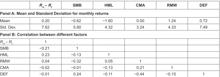
Panel A of Table 1 reports some descriptive statistics for the factors (independent variables) used in the analysis.

The time-series mean of the market risk premium, RMW

and DEF are all positive i.e., 0.2, 1.24 and 0.7 percent per

month, respectively. Conversely, the averages of SMB

(−0.62 percent per month) and HML (−1.6 percent per

month) are negative whereas CMA accounts on average

zero risk premium.

Panel B of Table 1 reports the correlation coefficients of the factors used in the current study. The highest correlation among any of the two factors is found between DEF and CMA (−0.44). The high (albeit negative) correlation indicates that DEF and CMA are closely associated and that variation in equity return explained by each factor is partially captured by the other. It is pertinent to note here that the DEF is created by independent sorts on the probability of default that is why DEF is relatively highly correlated with CMA. The creation of the default risk factor solely on the probability of default would allow us to draws a stronger conclusion regarding whether other factors are proxying default risk.

5.2. CMA: A Redundant Factor

Fama and French (2015) find the HML factor redundant in the presence of the remaining Fama-French four factors.

To examine whether a specific factor is explained by the remaining factors (including DEF), we run five-factor regressions to test whether it explains the sixth factor. To save space, we skip the results of these individual regressions.

The results for modelling the DEF risk factor on the Fama-French five factors reveal that the large average variation is mostly absorbed by CMA. The slope of CMA is strongly negative, which seems counterintuitive as it implies that firms with high default risk tend to invest aggressively when controlling other factors. Moreover, when regressing each factor on all other factors, the variation in the CMA regression is largely explained by SMB, RMW, and DEF.

The coefficients are somewhat contrasting with the economic rationale. For instance, a negative coefficient of SMB in CMA regression suggests that small stocks are found to be investing aggressively which happens generally when firms are in the growth stage. Whereas the positive

coefficient of RMW indicates that stocks of the firms with robust profitability behave like stocks with conservative investing which could be the case when firms are in a mature stage of their life cycle.

In the spirit of Fama and French (2015), therefore, we define CMAO (orthogonal CMA) as the sum of the intercept and residuals from a regression of CMA on R

− R

, SMB, HML, RMW, and DEF. Substituting CMAO for CMA in eq (2) produces an alternative version of the five-factor model:

r b r s h c

r d e

it i i mt i t i t i t

i t i t it

 SMB HML CMAO

RMW DEF (3)

The intercept and residuals are similar to that of equation (3), therefore, two regressions are equivalent for evaluating the model’s performance. The results in other sections are based on the orthogonal investment risk factor (i.e., CMAO).

5.3. Useless Factor Test

Another important concern is that a new factor may not be relevant across the test assets. Following Kan and Zhang (1999), we analyze whether the DEF factor is a ‘useless factor’ or adds value in asset pricing. In this regard, we jointly test whether DEF loadings are different from zero.

The wald-test rejects the hypothesis with p-values less than 0.01 across all sets of portfolios. Therefore, it can be concluded that none of the Fama-French five factors fully subsume the DEF factor. In other words, no convincing evidence is available for empirical replacement of default risk factor and it seems that DEF is capturing cross-sectional variations independently. Therefore, it justifies augmenting the five-factor model with the DEF factor.

Table 1: Descriptive Statistics for Factor Returns

R

– R

SMB HML CMA RMW DEF

Panel A: Mean and Standard Deviation for monthly returns

Mean 0.20 −0.62 −1.60 0.00 1.24 0.72

Std. Dev. 7.62 5.80 4.32 3.24 4.33 7.49

Panel B: Correlation between different factors

R

– R

1

SMB −0.21 1

HML 0.23 −0.13 1

RMW 0.04 −0.32 0.05 1

CMA −0.02 −0.01 −0.13 0.21 1

DEF −0.01 0.24 −0.11 −0.44 −0.15 1

Notes: Panel A of the table depicts descriptive statistics (mean, standard deviation, and t-statistics) for the excess market return as well as

returns on other factors employed. Panel B reports the correlation among these factors.

5.4. Model Performance Summary and Basic Regressions

We now compare how well the Fama-French five-factor model, as well as the augmented five-factor model, explain the average excess returns on the portfolios. We consider six asset pricing models including the five-factor model and the augmented five-factor for the full sample period (i.e., 2006–

2015), for the first sub-sample (i.e., 2006–09), and for the second sub-sample (i.e., 2010–2015). All these models are tested across all seven sets of portfolios. If the asset pricing model completely captures expected returns, the intercept term is indistinguishable from zero in the regression of the portfolio’s excess return on the factor return of the model.

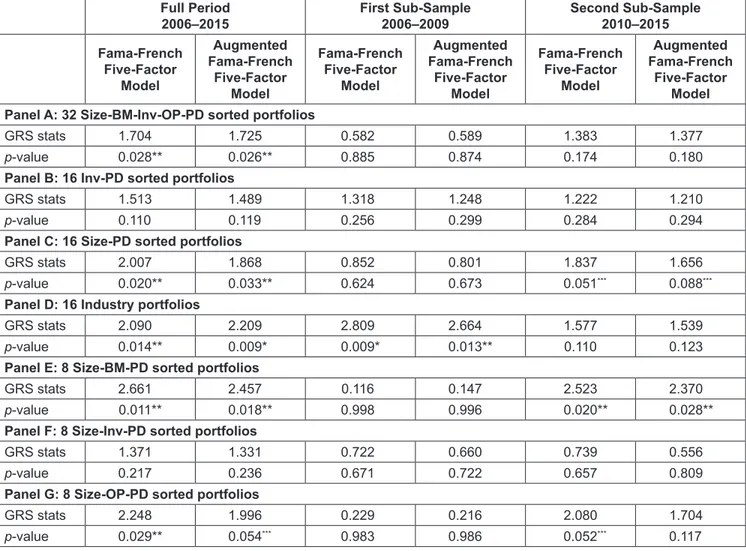
The GRS test statistics of Gibbons et al. (1989) presented in Table 2 does not reject the null hypothesis (i.e., the individual intercept coefficients are jointly equal to zero) for full sample and sub-samples across 16 Investment-PD and 8 Size-Inv-PD sorted portfolios for both Fama-French five-factor (FF5) and augmented five-factor models (AFF5). For industry portfolios, the GRS test accepts both FF5 and AFF5 for the second sub- sample only. Conversely, both models (FF5 and AFF5) only explain cross-sectional variation adequately for the first sample period, however, fail to retain the explanatory power in the second sub-sample and full sample period when tested across 16 Size-PD sorted, eight Size-BM-PD and eight Size-OP-PD sorted portfolios.

Table 2: Model Diagnostics: GRS Test Full Period

2006–2015 First Sub-Sample

2006–2009 Second Sub-Sample

2010–2015 Fama-French

Five-Factor Model

Augmented Fama-French

Five-Factor Model

Fama-French Five-Factor

Model

Augmented Fama-French

Five-Factor Model

Fama-French Five-Factor

Model

Augmented Fama-French

Five-Factor Model Panel A: 32 Size-BM-Inv-OP-PD sorted portfolios

GRS stats 1.704 1.725 0.582 0.589 1.383 1.377

p-value 0.028** 0.026** 0.885 0.874 0.174 0.180

Panel B: 16 Inv-PD sorted portfolios

GRS stats 1.513 1.489 1.318 1.248 1.222 1.210

p-value 0.110 0.119 0.256 0.299 0.284 0.294

Panel C: 16 Size-PD sorted portfolios

GRS stats 2.007 1.868 0.852 0.801 1.837 1.656

p-value 0.020** 0.033** 0.624 0.673 0.051

0.088

Panel D: 16 Industry portfolios

GRS stats 2.090 2.209 2.809 2.664 1.577 1.539

p-value 0.014** 0.009* 0.009* 0.013** 0.110 0.123

Panel E: 8 Size-BM-PD sorted portfolios

GRS stats 2.661 2.457 0.116 0.147 2.523 2.370

p-value 0.011** 0.018** 0.998 0.996 0.020** 0.028**

Panel F: 8 Size-Inv-PD sorted portfolios

GRS stats 1.371 1.331 0.722 0.660 0.739 0.556

p-value 0.217 0.236 0.671 0.722 0.657 0.809

Panel G: 8 Size-OP-PD sorted portfolios

GRS stats 2.248 1.996 0.229 0.216 2.080 1.704

p-value 0.029** 0.054

0.983 0.986 0.052

0.117

Notes: This table tests the ability of Fama-French five-factor and augmented Fama-French five-factor models to explain the monthly excess

return on 32 Size-BM-Inv-OP-PD portfolios (Panel A), 16 Inv-PD portfolios (Panel B), 16 Size-PD portfolios (Panel C), 16 Industry portfolios

(Panel D), 8 Size-BM-PD portfolios (Panel E), 8 Size-Inv-PD portfolios (Panel F), 8 Size-OP-PD portfolios (Panel E). Each Panel includes

GRS statistics and p-values for the full period (i.e. 2006–2015) as well as for both sub-periods. *, **, *** indicate statistical significance at 1,

5, and 10 percent levels, respectively.

To save space, results corresponding to basic Fama- French regressions are not shown. The highest average R

corresponds to 2 × 2 × 2 size-investment-PD sorted portfolios, i.e., 51.7 percent followed by 51.1 percent for 2 × 2 × 2 size- profitability-PD sorted portfolios.

5.5. Fama-MacBeth Regression Results

Tables 3 to 6 are presenting time-series averages of the slopes from the Fama-MacBeth (FM) month-by-month cross-sectional regressions of portfolio return on the market, size, value, investment, profitability, and default risk exposures. The average slopes provide the standard FM test for examining which factor has a statistically non-zero risk premium. Each table reports results for the full period as well as for two sub-periods divided at December 2009.

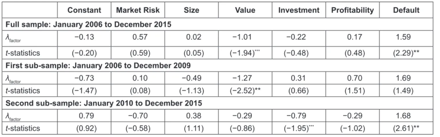
Table 3 provides the results of the regression for 32 size- value-profitability-investment-default sorted portfolios. The default risk premium is significantly positive with a monthly risk premium of 1.59 percent and 1.68 percent for the full sample period and second sub-period, respectively, whereas appears insignificant in the first sub-period. Notably, a significant default risk premium for the second sub-sample advocates the high default risk after the Global Financial Crisis of 2007–08. Moreover, there exists a significant negative risk premium for the value factor for the full sample period as well as for the first sub-period with average risk premiums of −1 percent and −1.27 percent per month, respectively.

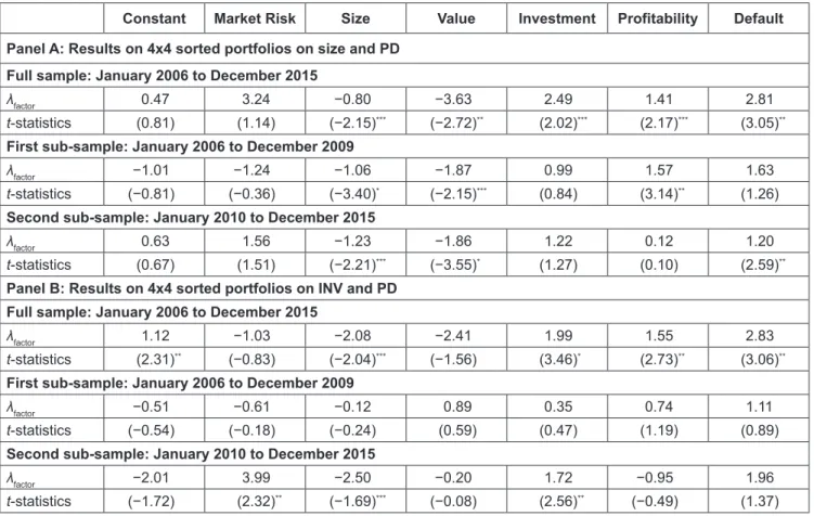
Panel A of Table 4 illustrates the results for 16 size- PD sorted portfolio regression. The default effect remains positive and statistically significant in the full sample period as well as in the second sub-period which implies that the default factor is priced in portfolio returns, thus, systematic in nature. Similarly, a risk premium for the profitability factor also appears positive and statistically significant for the full sample and first sub-period. Size and value factors command statistically significant, but negative risk premiums for the full period as well as for both subperiods. Moreover, risk premiums for investment and profitability risk factors are statistically meaningful for a full period, however, only the risk premium corresponds to profitability turn out significant for the first sub-sample.

For results corresponding to investment-PD sorted portfolios in Panel B of Table 4, CMAO, INV, and DEF have significantly positive factor premiums. In the second sub-period, premiums for market and investment factors turned out significantly positive. It is pertinent to note here that in the first sub-period, i.e., 2006 to 2009 none of the factor risk premiums are found significant.

Similarly, Table 5 contains the results of the 2 × 2 × 2 sorted portfolios. Panel A presents the results pertaining to sort on size, BM, and PD. It is evident that risk premiums for market, size, value and profitability factors appear statistically significant for a full sample period whereas size, value, investment, and profitability for the first sample period and market, size, and value for the second sample period earn significant risk premiums.

Table 3: Fama-MacBeth Regression Results - 2 × 2 × 2 × 2 × 2 Sorted Portfolios

Constant Market Risk Size Value Investment Profitability Default Full sample: January 2006 to December 2015

λ

−0.13 0.57 0.02 −1.01 −0.22 0.17 1.59

t-statistics (−0.20) (0.59) (0.05) (−1.94)

(−0.48) (0.48) (2.29)**

First sub-sample: January 2006 to December 2009

λ

−0.73 0.10 −0.49 −1.27 0.31 0.70 1.69

t-statistics (−1.47) (0.08) (−1.13) (−2.52)** (0.66) (1.51) (1.49)

Second sub-sample: January 2010 to December 2015

λ

0.79 −0.70 0.38 −0.29 −0.79 −0.29 1.68

t-statistics (0.92) (−0.58) (1.11) (−0.86) (−1.95)

(−1.02) (2.61)**

Notes: The table presents the average slopes (i.e., risk premiums) of cross-sectional regressions of Fama-MacBeth (1973) employed for the Fama-French five-factor model augmented with default factor (DEF) regressions on 32 SIZE, B/M, OP, PD, and INV sorted portfolios.

Newey-West heteroskedasticity and autocorrelated errors (HAC) adjusted t-statistics are reported in parenthesis. *, **, *** indicate statistical

significance at 1, 5, and 10 percent levels, respectively.

Table 4: Fama-MacBeth Regression Results - 4 × 4 Sorted Portfolios

Constant Market Risk Size Value Investment Profitability Default Panel A: Results on 4x4 sorted portfolios on size and PD

Full sample: January 2006 to December 2015

λ

0.47 3.24 −0.80 −3.63 2.49 1.41 2.81

t-statistics (0.81) (1.14) (−2.15)

(−2.72)

(2.02)

(2.17)

(3.05)

First sub-sample: January 2006 to December 2009

λ

−1.01 −1.24 −1.06 −1.87 0.99 1.57 1.63

t-statistics (−0.81) (−0.36) (−3.40)

(−2.15)

(0.84) (3.14)

(1.26)

Second sub-sample: January 2010 to December 2015

λ

0.63 1.56 −1.23 −1.86 1.22 0.12 1.20

t-statistics (0.67) (1.51) (−2.21)

(−3.55)

(1.27) (0.10) (2.59)

Panel B: Results on 4x4 sorted portfolios on INV and PD Full sample: January 2006 to December 2015

λ

1.12 −1.03 −2.08 −2.41 1.99 1.55 2.83

t-statistics (2.31)

(−0.83) (−2.04)

(−1.56) (3.46)

(2.73)

(3.06)

First sub-sample: January 2006 to December 2009

λ

−0.51 −0.61 −0.12 0.89 0.35 0.74 1.11

t-statistics (−0.54) (−0.18) (−0.24) (0.59) (0.47) (1.19) (0.89)

Second sub-sample: January 2010 to December 2015

λ

−2.01 3.99 −2.50 −0.20 1.72 −0.95 1.96

t-statistics (−1.72) (2.32)

(−1.69)

(−0.08) (2.56)

(−0.49) (1.37)

Notes: The table presents the average slopes (i.e. risk premiums) of cross-sectional regressions of Fama-MacBeth (1973) employed for the Fama-French five-factor model augmented with default factor (DEF) regressions on 4x4 sorted portfolios on size and PD (panel A) as well as INV and PD (panel B). Newey-West heteroskedasticity and autocorrelated errors (HAC) adjusted t-statistics are reported along with risk premiums. *, **, *** indicate statistical significance at 1, 5, and 10 percent levels, respectively.

Results in panel B of Table 5 corresponds to the eight size-investment-PD sorted portfolios. All five factors and default risk factor command significant risk premiums for the full period and second sample period. In the first sub-sample, size, investment, and default risk factors are statistically significant. Notably, the alpha risk premium is also statistically significant for the full period and for both sub-periods suggesting potential mispricing. Also, panel C illustrates results on portfolio sorts on size, profitability and probability of default. It is found that risk premiums for size, profitability and default risk factors turn out statistically significant for the full sample period, however, the risk premiums for size and profitability factor appears significant in the second sub-period whereas size and value factors earn significant risk premiums in first sample sub-period.

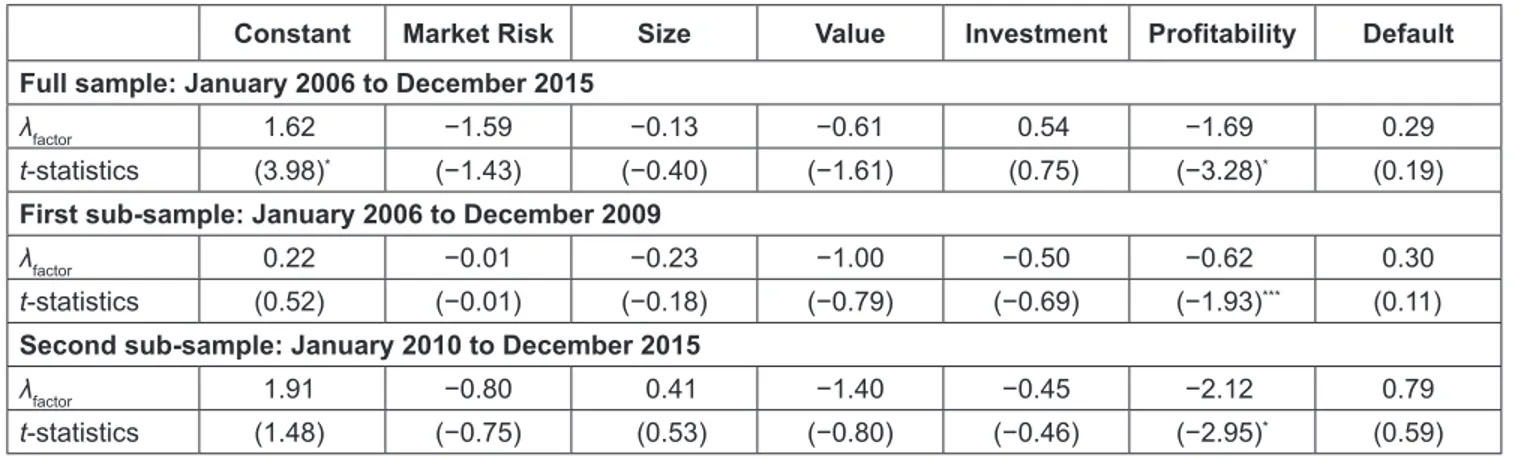
Similarly, results on factor risk premiums for industry portfolios are reported in Table 6. The expected risk

premiums are somehow contradictory as compared with previous sorting techniques. Profitability (RMW) risk factor is effectively priced in full period and first sample period whereas default risk is not found systematic in any sample period for industry portfolios.

All other factor risk premiums in full or sub-period are

statistically insignificant. The risk premiums for RMW

is around −1.7 percent, −0.6 percent and −2.1 percent

per month for the full period, first, and second sample

period respectively, suggesting a healthy premium for the

profitability risk factor. Previous studies (such as Fama and

French, 1997) find that Fama-French three factors do not

perform well in explaining equity returns when industry-

based portfolios are employed, this study brings evidence

that the five-factor model along with additional default risk

factor also does not add much value in explaining variation

across industry portfolios.

Table 5: Fama-MacBeth Regression Results - 2 × 2 × 2 Sorted Portfolios

Constant Market Risk Size Value Investment Profitability Default Panel A: Results on 2 × 2 × 2 sorted portfolios on size, BM and PD

Full sample: January 2006 to December 2015

λ

3.67 −6.62 −1.73 −3.36 0.34 −5.61 1.29

t-statistics (4.66)* (−3.29)* (−8.48)* (−22.2)* (0.31) (−2.47)* (1.17)

First sub-sample: January 2006 to December 2009

λ

0.78 −0.42 −0.84 −2.98 −1.73 1.01 −0.01

t-statistics (3.54)* (−1.29) (−15.0)* (−17.5)* (−5.25)* (5.95)* (−0.02)

Second sub-sample: January 2010 to December 2015

λ

1.07 −3.38 −1.57 −1.79 −6.40 −7.37 −0.30

t-statistics (0.60) (−3.23)* (−2.92)* (−3.23)* (−1.55) (−0.97) (−0.51)

Panel B: Results on 2 × 2 × 2 sorted portfolios on Size, INV and PD Full sample: January 2006 to December 2015

λ

−6.39 11.1 −2.95 5.84 0.57 −5.79 5.91

t-statistics (−45.6)* (53.9)* (−61.9)* (34.8)* (14.8)* (−51.0)* (53.2)*

First sub-sample: January 2006 to December 2009

λ

−1.39 0.93 −2.04 −0.33 1.01 −0.41 2.36

t-statistics (−2.29)* (0.42) (−8.97)* (−0.41) (8.70)* (−1.17) (4.78)*

Second sub-sample: January 2010 to December 2015

λ

2.93 −1.39 0.18 −4.48 1.26 2.61 1.54

t-statistics (78.6)* (−36.0)* (28.6)* (−146)* (54.7)* (59.8)* (61.8)*

Panel C: Results on 2 × 2 × 2 sorted portfolios on Size, OP and PD Full sample: January 2006 to December 2015

λ

−0.94 1.26 −0.97 −0.88 −1.77 2.44 1.43

t-statistics (−1.20) (0.39) (−2.09)* (−0.38) (−0.89) (2.44)* (2.77)*

First sub-sample: January 2006 to December 2009

λ

−0.72 −1.90 −1.04 −2.22 0.26 1.33 −0.34

t-statistics (−0.47) (−0.99) (−2.64)* (−1.76)** (0.23) (1.46) (−0.21)

Second sub-sample: January 2010 to December 2015

λ

0.28 −0.05 −0.87 −0.61 −1.76 2.17 1.40

t-statistics (0.19) (−0.01) (−4.03)* (−0.33) (−0.73) (2.19)* (1.02)

Notes: The table represents the average slopes (i.e. risk premiums) of cross-sectional regressions of Fama-MacBeth (1973) employed for

Fama-French five-factor model augmented with default factor (DEF) regressions on 2 ×2 ×2 sorted portfolios on size, BM, PD (panel A) as

well as INV and PD (panel B). Newey-West heteroskedasticity and autocorrelated errors (HAC) adjusted t-statistics (in parenthesis) are

reported along with risk premiums. *, **, *** indicate statistical significance at 1, 5, and 10 percent levels, respectively.

6. Conclusion

This study aims to test the ‘distress hypothesis’, i.e., size and book-to-market factors proxy default risk factor as contended by previous studies such as Fama and French (1992, 1996). However, the superior measure of default risk is required in order to construct a default risk factor. This paper uses a hybrid-ANN model to compute the probability of default which has attained a higher level of predictive accuracy for the non-financial sector of Pakistan (see Khan et al., 2020). This study extends the existing literature by testing whether Fama-French five factors proxy default risk and nature of default risk factor are examined in the five-factor asset pricing framework. It examines the performance of the augmented Fama-French five model across different sets of portfolios and tested temporal stability. To serve this purpose, the study uses three portfolio sorting approaches based on financial characteristics apart from industry portfolios and temporal stability is examined by splitting the full sample into two sub-sample periods: 2005–2009 and 2010–2015.

Our findings suggest that default risk is priced in equity returns, therefore, systematic, which is in line with Griffin and Lemmon (2002), Vassalou and Xing (2004), and others.

We found that the estimated factor premium on default risk is significantly positive for most of the cases except industry portfolios. Moreover, we reject the notion that the DEF is ‘useless’ and also reject the hypothesis that default risk is explained by any of the Fama-French five factors.

However, the investment factor (i.e. CMA) contains some information but a separate and independent role of the default risk factor is statistically pronounced. We control the negative correlation found between investment (CMA) and default (DEF) risk factors by using orthogonalized CMA. It can be concluded that default is a factor worth considering

in asset-pricing tests beyond size, value, profitability, and investment risk factors.

The highest average R

(i.e., 52 percent) is found when portfolios are sorted on proxies of size, investment, and default risk. It implies that the augmented five-factor model has a relatively greater predictive ability when implied for the aforementioned sorting approach. One could suggest that practitioners can benefit from this model if they can convert stocks into 2 × 2 × 2 Size-Inv-PD sorted portfolios. Moreover, the significance of the default risk factor for full-sample as well as both sub-samples are highly pronounced in this model endorsing the temporal stability of the factor.

In addition, the GRS test also accepts both Fama-French five-factor and augmented Fama-French five-factor models for explaining cross-sectional returns when tested across 2 × 2 × 2 Size-Inv-PD sorted portfolios.

Collectively, our evidence suggests a systematic relation between expected returns and default risk.

Surprisingly, firms having high bankruptcy risk earning a lower realized return and a risk-based explanation do not explain the anomalous evidence of bankruptcy risk. The results of this study would encourage investors to require additional default risk premium, thus, anomalous relation between realized return and risk could be corrected. As a company gets into financial distress, the investors often react to the chances of default by selling stocks of distressed companies that drag down the price of these securities.

These distressed stocks are attractive for bargain investors who are willing to accept a significant risk and possess a somewhat different perspective on the firm from market participants. Because of the high degree of risk involved, distressed stocks are attractive investment venue for large institutional investors such as private equity funds, hedge funds, and investment banks.

Table 6: Fama-MacBeth Regression Results - Industry Portfolios

Constant Market Risk Size Value Investment Profitability Default Full sample: January 2006 to December 2015

λ

1.62 −1.59 −0.13 −0.61 0.54 −1.69 0.29

t-statistics (3.98)

(−1.43) (−0.40) (−1.61) (0.75) (−3.28)

(0.19)

First sub-sample: January 2006 to December 2009

λ

0.22 −0.01 −0.23 −1.00 −0.50 −0.62 0.30

t-statistics (0.52) (−0.01) (−0.18) (−0.79) (−0.69) (−1.93)

(0.11)

Second sub-sample: January 2010 to December 2015

λ

1.91 −0.80 0.41 −1.40 −0.45 −2.12 0.79

t-statistics (1.48) (−0.75) (0.53) (−0.80) (−0.46) (−2.95)

(0.59)

Notes: The table presents the average slopes (i.e., risk premiums) of cross-sectional regressions of Fama-MacBeth (1973) employed for the

Fama-French five-factor model augmented with default factor (DEF) regressions on 16 industry portfolios. Newey-West heteroskedasticity

and autocorrelated errors (HAC) adjusted t-statistics are reported along with risk premiums. *, **, *** indicate statistical significance at 1

percent, 5 percent, and 10 percent levels, respectively.

References

Agarwal, V., & Taffler, R. (2008). Does financial distress risk drive the momentum anomaly? Financial Management, 37(3), 461–484. https://www.jstor.org/stable/20486664

Altman, E. I. (1968). Financial ratios, discriminant analysis and the prediction of corporate bankruptcy. The Journal of Finance, 23(4), 589–609. https://doi.org/10.2307/2978933

Altman, E. I., & Rijken, H. A. (2011). Toward a bottom-up approach to assessing sovereign default risk. Journal of Applied Corporate Finance, 23(1), 20–31. https://doi.org/10.1111/

j.1745-6622.2011.00311.x

Ang, A., Liu, J., & Schwarz, K. (2010). Using stocks or portfolios in tests of factor models. Journal of Financial and Quantitative Analysis, 1–42.

Asis, G., Chari, A., & Haas, A., 2020. In search of distress risk in emerging markets. NBER Working Paper 27213. https://doi.

org/10.0.13.58/w27213

Avramov, D., & Zhou, G. (2010). Bayesian portfolio analysis.

Annual Review of Financial Economics, 2(1), 25–47. https://

doi.org/10.1146/annurev-financial-120209-133947

Bauer, J. (2012). Bankruptcy risk prediction and pricing:

Unravelling the negative distress risk premium. Bedford, UK:

Doctoral dissertation, Cranfield University. https://dspace.lib.

cranfield.ac.uk/handle/1826/7313

Campbell, J. Y., Hilscher, J., & Szilagyi, J. (2008). In search of distress risk. The Journal of Finance, 63(6), 2899–2939. https://

doi.org/10.1111/j.1540-6261.2008.01416.x

Chan, H., Faff, R., & Kofman, P. (2011). Is default risk priced in Australian equity? Exploring the role of the business cycle.

Australian Journal of Management, 36(2), 217–246. https://

doi.org/10.1177%2F0312896211407528

Chan, K. C., & Chen, N. F. (1991). Structural and return characteristics of small and large firms. The Journal of Finance, 46(4), 1467–1484. https://doi.org/10.1111/j.1540-6261.1991.

tb04626.x

Chen, N. F., & Zhang, F. (1998). Risk and return of value stocks. The Journal of Business, 71(4), 501–535. https://doi.

org/10.1086/209755

Dichev, I. D. (1998). Is the risk of bankruptcy a systematic risk?

The Journal of Finance, 53(3), 1131–1147. https://doi.

org/10.1111/0022-1082.00046

Drobetz, W., Sturmer, S., & Zimmermann, H. (2002). Conditional asset pricing in emerging stock markets. The Swiss Journal of Economics and Statistics, 138(4), 507–526. http://www.sjes.ch/

papers/2002-IV-11.pdf

Fama, E. F., & French, K. R. (1992). The cross-section of expected stock returns. The Journal of Finance, 47(2), 427–465. https://

doi.org/10.1111/j.1540-6261.1992.tb04398.x

Fama, E. F., & French, K. R. (1993). Common risk factors in the returns on stocks and bonds. Journal of Financial Economics, 33(1), 3–56.

Fama, E. F., & French, K. R. (1996). Multifactor explanations of asset pricing anomalies. The Journal of Finance, 51(1), 55–84.

https://doi.org/10.1111/j.1540-6261.1996.tb05202.x

Fama, E. F., & French, K. R. (1997). Industry costs of equity.

Journal of Financial Economics, 43(2), 153–193. https://doi.

org/10.1016/S0304-405X(96)00896-3

Fama, E. F., & French, K. R. (2015). A five-factor asset pricing model. Journal of Financial Economics, 116(1), 1–22. https://

doi.org/10.1016/j.jfineco.2014.10.010

Fama, E. F., & French, K. R. (2016). Dissecting anomalies with a five-factor model. The Review of Financial Studies, 29(1), 69–103. https://doi.org/10.1093/rfs/hhv043

Fama, E. F., & MacBeth, J. D. (1973). Risk, return, and equilibrium: Empirical tests. Journal of Political Economy, 81(3), 607–636. https://www.journals.uchicago.edu/doi/

abs/10.1086/260061

Foye, J. (2018). A comprehensive test of the Fama-French five-factor model in emerging markets. Emerging Markets Review, 37, 199–222. https://doi.org/10.1016/j.ememar.2018.

09.002

Gharghori, P., Chan, H., & Faff, R. (2007). Are the Fama- French factors proxying default risk? Australian Journal of Management, 32(2), 223–249. https://doi.org/10.1177%

2F031289620703200204

Gharghori, P., Chan, H., & Faff, R. (2009). Default risk and equity returns: Australian evidence. Pacific-Basin Finance Journal, 17(5), 580–593. https://doi.org/10.1016/j.pacfin.2009.03.001 Gibbons, M. R., Ross, S. A., & Shanken, J. (1989). A test of

the efficiency of a given portfolio. Econometrica: Journal of the Econometric Society, 57(5), 1121–1152. https://doi.

org/10.2307/1913625

Griffin, J. M., & Lemmon, M. L. (2002). Book-to-market equity, distress risk, and stock returns, The Journal of Finance, 57(5), 2317–2336. https://doi.org/10.1111/1540-6261.00497

Hoang, L. T., Phan, T. T., & Ta, L. N. (2020). Nominal Price Anomaly in Emerging Markets: Risk or Mispricing? Journal of Asian Finance, Economics and Business, 7(9), 125–134.

https://doi.org/10.13106/jafeb.2020.vol7.no9.125

Iqbal, J. (2012). Stock market in Pakistan: An overview. Journal of Emerging Market Finance, 11(1), 61–91. https://doi.org/10.117 7%2F097265271101100103

Iqbal, J., Brooks, R., & Galagedera, D. U. (2010). Testing conditional asset pricing models: An emerging market perspective. Journal of International Money and Finance, 29(5), 897–918. https://

doi.org/10.1016/j.jimonfin.2009.12.004

Kan, R., & Zhang, C. (1999). Two‐pass tests of asset pricing models with useless factors. The Journal of Finance, 54(1), 203–235.

https://doi.org/10.1111/0022-1082.00102

Khan, U. E., Iqbal, J., & Iftikhar, F. (2020). The Riskiness of Risk Models: Assessment of Bankruptcy Risk of Non-Financial Sector of Pakistan, Business & Economic Review, 12(2). http://

dx.doi.org/10.22547/BER/12.2.3

Lo, A. W., & MacKinlay, A. C. (1990). Data-snooping biases in tests of financial asset pricing models. The Review of Financial Studies, 3(3), 431–467. https://doi.org/10.1093/

rfs/3.3.431

Modigliani, F., & Miller, M. H. (1958). The cost of capital, corporation finance and the theory of investment. The American Economic Review, 48(3), 261–297. https://www.jstor.org/

stable/1809766

Nurhayati, I., & Endri, E. (2020). A New Measure of Asset Pricing:

Friction-Adjusted Three-Factor Model. Journal of Asian Finance, Economics and Business, 7(12), 605–613. https://doi.

org/10.13106/jafeb.2020.vol7.no12.605

Ohlson, J. A. (1980). Financial ratios and the probabilistic prediction of bankruptcy. Journal of Accounting Research, 18(1), 109–131. https://doi.org/10.2307/2490395

Pojanavatee, S. (2020). Tests of a Four-Factor Asset Pricing Model: The Stock Exchange of Thailand. Journal of Asian

Finance, Economics and Business, 7(9), 117–123. https://doi.

org/10.13106/jafeb.2020.vol7.no9.117

Shleifer, A., & Vishny, R. W. (1997). A survey of corporate governance. The Journal of Finance, 52(2), 737–783. https://

doi.org/10.1111/j.1540-6261.1997.tb04820.x

Vassalou, M., & Xing, Y. (2004). Default risk in equity returns. The Journal of Finance, 59(2), 831–868. https://doi.org/10.1111/j.

1540-6261.2004.00650.x

Endnotes

1

The probability of default estimates is obtained from a hybrid of dynamic panel probit and artificial neural network model. See Khan Iqbal and Iftikhar (2020) for details.

2

For details see Khan, Iqbal and Iftikhar (2020).

3

n.e.s stands for not elsewhere specified.