MATLAB을 이용한 Condensation 알고리즘의 자동 코드 구현
Development of Automatic Code Generation of Condensation Algorithm using MATLAB
이양원* Yang-Weon Lee*
요 약
본 논문에서는 다중물체를 추적하기 위해서 적합한 것으로 알려진 condensation 알고리즘의 자동 코드 발생 기를 연구한 결과를 보인 것이다. 일반적으로 condensation 알고리즘은 일반인이 구현하기 매우 어려워 실제 유비쿼터스 상황인지를 위하여 필요한 기술임에도 불구하고 널리 이용되지 못하고 있다. 본 논문에서는 이 같 은 문제점을 개선하기 위하여 시스템 다이나믹스 모델과 측정 모델이 주어지면 요구하는 성능을 만족하는 condensation algorithm이 내장된 필터를 자동으로 만들어주는 MATLAB 코드를 발생하도록 설계하였다. 일단 발생된 MATLAB 코드는 C, C++ 언어 등으로 변환되므로 원하는 소스를 얻을 수 있다.
Abstract
This paper address the problem of tracking multiple objects encountered in many situations in developing condensation algorithms. The difficulty lies on the fact that the implementation of condensation algorithm is not easy for the general users. We propose an automatic code generation program for condensation algorithm using MATLAB tool. It will help for general user who is not familiar with condensation algorithm to apply easily for real system. The merit of this program is that a general industrial engineer can easily simulate the designed system and confirm the its performance on the fly.
Key words : multiple target tracking(다중표적추적), Condensation algorithm(컨덴세이션 알고리즘), particle filter(입자필터), code generation(코드 발생기), Matlab(매트랩)
* 호남대학교 정보통신공학과 ‧ 제1저자 (First Author) : 이양원 ‧ 투고일자 : 2010년 8월 26일
‧ 심사(수정)일자 : 2010년 8월 27일 (수정일자 : 2010년 10월 25일) ‧ 게재일자 : 2010년 10월 30일
I. Introduction
Multiple object tracking(MTT) deals with state estimation of an unknown number of moving targets.
Available measurements may both arise from the targets if they are detected, and from clutter. Clutter is generally
considered as a model describing false alarms. Its (spatio-temporal) statistical properties are quite different from target ones, which makes possible the extraction of target tracks from clutter. To perform multiple object tracking the observer has at his disposal a huge amount of data, possibly collected on multiple receivers. In
signal processing, elementary measurements are receiver outputs, e.g., bearings, ranges, time delays, Dopplers, etc. In image-based tracking they have to be computed from the images. But the main difficulty comes from the assignment of a given measurement to a target model[1].
These assignments are generally unknown, as are the true target models. This is a neat departure from classical estimation problems[2]. Thus, two distinct problems have to be solve it jointly: data association and estimation. As long as the association is considered in a deterministic way, the hypothesis associations must be exhaustively enumerated, which leads to a NP hard problem (as in JPDAF and MHT algorithms[3] for instance). As soon as the association variables are considered as stochastic variables and moreover statistically independent like in the Probabilistic MHT (PMHT), the complexity is reduced[4]. However, the above algorithms do not cope with non linear state or measurement models and non Gaussian state or measurement noises. Under such assumptions (stochastic state equation and non linear state or measurement equation, non Gaussian noises), particle filters are particularly adapted[5]. They mainly consist in propagating a weighted set of particles which approximates the probability density of the state conditionally to the observations. Particle filtering can be applied under very weak hypotheses, is able to cope with heavy clutter, and is very easy to implement\cite[6].
Numerous versions have been used in various contexts:
the bootstrap filter for target tracking in [7], the Condensation algorithm in image analysis are two examples among others. In image analysis a probabilistic exclusion principle has been developed in [5] to track multiple objects but the algorithm is very dependent on the observation model and seems costly to extend for more than two objects. We propose here a quite general algorithm for multiple object tracking applicable both in signal and image analysis.
The tracking system for the ubiquitous application is shown in Fig.1
This paper is organized as follows. In section II, we briefly recall the basic particle condensation filter.
Section III deals with structure of the generated program to multiple objects. Section IV begins with a validation of our program.
그림 1. 유비쿼터스를 위한 추적 시스템 구성도 Fig. 1. Tracking system configuration for ubiquitous
Ⅱ. Condensation Algorithm
2-1 Particle Filter
For the sake of completeness, the basic particle filter is now briefly reviewed. The particle filter approach to track multiple targets, also known as the condensation algorithm[5] and Monte Carlo localization [4], uses a large number of particles to explore the state space.
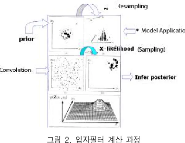
Each particle represents a hypothesized target location in state space. Initially the particles are uniformly randomly distributed across the state space, and each subsequent frame the algorithm cycles through the steps illustrated in Fig.2 :
① Deterministic drift: particles are moved according to a deterministic motion model (a damped constant velocity motion model was used).
② Update probability density function(PDF) : Determine the probability for every new particle location.
③ Resample particles: 90% the particles are
∊ m ax
∊
m in m ax
∊ m inm ax
(1) resampled with replacement, such that the probability of
choosing a particular sample is equal to the PDF at that point; the remaining 10% of particles are distributed randomly throughout the state space.
④ Diffuse particles: particles are moved a small distance in state space under Brownian motion.
그림 2. 입자필터 계산 과정 Fig. 2. Particle Filter Calculation Process
This results in particles congregating in regions of high probability and dispersing from other regions, thus the particle density indicates the most likely target states.
See [3] for a comprehensive discussion of this method.
The key strengths of the particle filter approach to localization and tracking are its scalability (computational requirement varies linearly with the number of particles), and its ability to deal with multiple hypotheses (and thus more readily recover from tracking errors). However, the particle filter was applied here for several additional reasons:
• It provides an efficient means of searching for a target in a multi-dimensional state space.
• Reduces the search problem to a verification problem, ie. is a given hypothesis face-like according to the sensor information?
• Allows fusion of cues running at different frequencies.
2-2 Application of Condensation Filter for the Ubiquitous Application
In order to apply the Condensation Algorithm to multitarget tracking , we extend the methods described by Black and Jepson [6]. Specifically, a state at time is described as a parameter vector: where: is the integer index of the predictive model,
indicates the current position in the model, refers to an amplitudal scaling factor and is a scale factor in the time dimension. Note that indicates which hand’s motion trajectory this , , or refers to left and right hand where ∊ . My models contain data about the motion trajectory of both the left hand and the right hand; by allowing two sets of parameters, I allow the motion trajectory of the left hand to be scaled and shifted separately from the motion trajectory of the right hand (so, for example, refers to the current position in the model for the left hand’s trajectory, while refers to the position in the model for the right hand’s trajectory). In summary, there are 7 parameters that describe each state.
Initialization : The sample set is initialized with N samples distributed over possible starting states and each assigned a weight of
. Specifically, the initial
parameters are picked uniformly according to:
Prediction : In the prediction step, each parameter of a randomly sampled is used to determine based on the parameters of that particular st . Each old state,, is randomly chosen from the sample set, based on the weight of each sample. That is, the weight of each sample determines the probability of its being
chosen. This is done efficiently by creating a cumulative probability table, choosing a uniform random number on [0, 1], and then using binary search to pull out a sample.
The following equations are used to choose the new state :
(2)
where refers to a number chosen randomly according to the normal distribution with standard deviation . This adds an element of uncertainty to each prediction, which keeps the sample set diffuse enough to deal with noisy data. For a given drawn sample, predictions are generated until all of the parameters are within the accepted range. If, after, a set number of attempts it is still impossible to generate a valid prediction, a new sample is created according to the initialization procedure above.
Updating : After the Prediction step above, there exists a new set of predicted samples which need to be assigned weights. The weight of each sample is a measure of its likelihood given the observed data
⋯. We define ⋯
as a sequence of observations for the th coefficient over time; specifically, let , , , be the sequence of observations of the horizontal velocity of the left hand, the vertical velocity of the left hand, the horizontal velocity of the right hand, and the vertical velocity of the right hand respectively.
Extending Black and Jepson [1], we then calculate the weight by the following equation:
⊓ (3)
where
and
where is the size of a temporal window that spans back in time. Note that , and refer to the appropriate parameters of the model for the blob in question and that
refers to the value given to the th coefficient of the model interpolated at time and scaled by .
Ⅲ. Automatic Code Generation
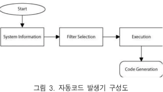
Automated code generation program is implemented by MATLAB and its toolbox packages. As shown in Figure 3, A program user only input the system information(system dynamics and measurement equation) into the program interactively. And then finally can get the particle filter code and using generated code also can execute the filter sequently.
그림 3. 자동코드 발생기 구성도 Fig. 3 Structure of automatic code generation
Its features include as following:
• This program have two parts : Implementation of filtering algorithm and its use.
• Major algorithm and options have been implemented using Condensation algorithm, Particle Filter EKF(Extended Kalman Filter), MM Particle Filter, Regularized Particle Filter, and Auxiliary Variable Particle Filter. To switch from one filter to another, user only needs to change a few lines of code that initialize the filtering objects. The code that performs the actual filtering need not be changed.
• A GUI(Graphical User Interface) is also implemented so that choices of filters with relevant
options can be made in an easy action.
3-1 Generation of Gaussian Distribution
In order to generate Gaussian Distribution, we used existing AWGN, WGN and GAUSS2MF in MATLAB toolbox. WGN Generate white Gaussian noise.
Y = WGN(M,N,P,IMP,STATE) resets the state of RANDN to STATE. P specifies the power of the output noise in dBW. Additional flags that can follow
the numeric arguments are: Y = WGN(..., POWERTYPE) specifies the units of P. POWERTYPE can be 'dBW', 'dBm' or 'linear'. Linear power is in Watts.
Y = WGN(..., OUTPUTTYPE); Specifies the output type. OUTPUTTYPE can be real or complex. If the output type is complex, then P is divided equally between the real and imaginary components.
3-2 Generation of Filter Code Blocks
We consider nonlinear discrete time systems with additive noises, in the following form
(4)
where is the state, is the measurement,
and are iid. noises, and ∊. From a simulation point of view, a filter is a dynamical system in the form
(5)
where is the internal state of the filter,
is the estimate of the current state based on the posterior distribution obtained by the filter, and the functions and are parameterized by the functions , , and statistics of ,
and . In other words, a filtering subsystem, for a
given system (4), takes in an observation and produces an estimate , based upon its internal state
, and the particular filtering algorithms used. In the case of Extended Kalman Filter, includes the estimated mean and covariance. In the case of a Particle Filter, includes all the particles and their weights, among others.
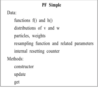
It therefore follows that we can use a MATLAB object to represent such a filter. An illustration of the PF Simple class in PFLib is shown in Figure 4. To use a filtering object, first we create one by choosing a desired class and properly initializing it:
>> aFilterObj = Particle_Filter_Class(initializing_parameters ...)
Then we can simply use it as follows:
>> for k = 1:Tmax
>> %%% other code omitted
>> aFilterObj = update(aFilterObj, y(k), ...);
>> xhat(k) = get(aFilterObj);
>> end
Here in each iteration, the lter object is updated with the new measurement. The get function can return particles and weights, as well as the state estimate.
PF Simple Data:
functions f() and h() distributions of v and w particles, weights
resampling function and related parameters internal resetting counter
Methods:
constructor update get
그림 4. 입자필터 구현 블록 내용 FIg. 4. Contents of particle filter
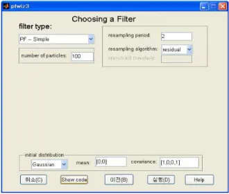
3-3 GUI Program
We have implemented the Bootstrap Particle Filter, the Particle Filter with an EKF-type, the Auxiliary Particle Filter, and the Instrumental Variable Particle Filter. Resampling scheme choices that we have implemented include (i)None (for pedagogical purpose), (ii)Simple Resampling, (iii)Residual Resampling, (iv)Branch-and-Kill, and (v)System Resampling. Other available choices include (i)sampling frequency, (ii)number of particles, and (iii)Jacobians.
Given the above options, initializing a particle filter object can become tedious - one would have to read the documentation and understand how each option is specified. To ease the user's burden, we have created a Graphical User Interface that first lets the user pick and choose and then generates the initialization code for the user. To illustrate, two screen shots are shown in Figures 5 and 6, with the former showing how information about the system is collected, and the latter, the filter.
그림 5 시스템 입력 GUI 창 Fig.5 GUI window of system information
IV. Experiment Result
To test the proposed program, we used two models, one dimension and two dimension system. The coefficient of filter are selected as shown in Fig. 5. After
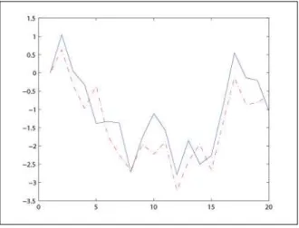
the user has made all the choices, initialization code will be shown in an editor window, as is displayed in Figure 6. Fig. 7 shown the generated code after program execution. Finally, Fig. 8 and 9 show tracking performances in derived filter using generated code.
그림 6 필터 정보 입력 GUI 창 Fig. 6 GUI window of filter information
그림 7 자동 코드 생성 결과
Fig. 7 Result of automatic code generation
V. Conclusions
In this paper, we have developed the automatic code
generation of particle filter for the ubiquitous application. This program is important in providing a general user to confirm the performance easily in design phase and also extend to include more or new filtering algorithms. We have proved that given a system dynamics and measurement information, automatic code generation program operate well in real environment.
그림 8 1차원 표적 추적 결과
Fig. 8 Tracking result of one dimension target
그림 9 2차원 표적 추적 결과
Fig. 9 Tracking result of two dimension target
References
[1] T. E. Fortmann, Y. Bar-Shalom, and M. Scheffe. Sonar
tracking of multiple targets using joint probabilistic data association. IEEE Journal of Oceanic Engineering, 173-184, July, 1983
[2] N. Gordon, D. Salmond, and A. Smith. Novel approach to nonlinear/non-Gaussian Bayesian state estimation.
IEE Proc.F, Radar and signal procesing, 107-113, 1993 [3] M. Isard and A. Blake. CONDENSATION . conditional
density propagation for visual tracking. Int. J.
Computer Vision, 5-28, 1998
[4] J. MacCormick and A. Blake. A probabilistic exclusion principle for tracking multiple objects. In Proc. Int.
Conf. Computer Vision, 572-578, 1999
[5] M.ISard and A.Blake: CONDENSATION-conditional density propagation for visual tracking. International Jour al of Computer Vision,29(1) 5-28, 1998 [6] Michael Isard and Andrew Blake: A mixed-state
condensation tracker with automatic model-switching,In Proceedings 6th International Conference of Computer Vision, 1998
[7] Yang Weon Lee, Adaptive Data Association for Multi-target Tracking using relaxation, LNCS 35644, 552-561, 2005.
이 양 원 (李陽源)
He Received B.S degree in the Dept. of Electrical Engineering from Chungang University, Korea, in 1982, and the M.S. degree in the Department of Control and Measurement Engineering from Seoul National University, in 1991. In 1996, he received Ph. D. degrees in the Dept. of Electrical Engineering from POSTECH, Korea. During 1982-1996, he worked for ADD as senior researcher. Since 1996, he has worked in the Dept. of Information and Communication Engineering at the Honam University, where he now works as a professor. His current research interests include smart computing, target estimation and tracking filter design, communication signal processing, and .NET application.