Ownership Structure and Performances: An Analysis of Cooperatives and Investor-Owned Utilities in the U.S.
Electric Power Industry
Heesun Jang*
ABSTRACT : This study examines performances of cooperatives relative to investor-owned firms in the US electric power industry. Using a panel data of firms from 2001 to 2014, the results show that cooperatives operate under conditions of more difficult capital constraints associated with the higher cost of debt and limited access to external equity capital. While investor-owned utilities, especially the large utilities that are less capital constrained, take benefits from substantial scale economies existing in the industry, the marginal cost of operation substantially increases with output for cooperatives. I do not find differences in profitability between the two ownership structures, measured by return on assets and return on equity. Plant capacity utilization, which is a measure of plant efficiency conditional on the operation, is also not statistically different between the two groups.
Keywords : Cooperatives, Marginal costs, Firm performances, Electric power industry
JEL 분류 : Q40, L10
Received: December 29, 2017. Revised: February 5, 2018. Accepted: February 8, 2018.
* Associate Research Fellow, Korea Energy Economics Institute, Corresponding author
(e-mail: [email protected])
운영성과의 차이 분석
장희선
*
요 약 : 본 연구는 미국 전력산업에서 협동조합과 민영전기사업자간의 소유권 형태의 차이가 기업의 운영성과에 미치는 영향을 분석한다. 2001년부터 2014년까지의 패널데이타를 구축하 여 비용함수, 이중차분법 등을 추정한 결과, 협동조합은 높은 이자비용과 제한된 자금조달 등 소유권 형태로 인해 자본이용에 제한이 있고 운영한계비용 또한 기업 규모에 따라 가파르게 증가하는 반면, 민영전기사업자의 경우 상대적으로 자유로운 자본접근성을 바탕으로 전력산업 에 존재하는 규모의 경제를 잘 활용하고 있는 것으로 분석되었다. 그러나 본 연구에서 소유권 형태가 기업의 수익성에 미치는 영향은 찾지 못하였으며, 발전효율성과 소유권형태의 상관관계 또한 통계적으로 유의미하지 않은 것으로 분석되었다.
주제어 : 전력협동조합, 한계비용, 운영성과, 미국 전력산업
접수일(2017년 12월 29일), 수정일(2018년 2월 5일), 게재확정일(2018년 2월 8일)
* 에너지경제연구원, 부연구위원, 교신저자(e-mail: [email protected])
I. Introduction
The purpose of this paper is to investigate the effects of ownership structure on firm performances in the context of the US electric power industry. In principal, differences in ownership structure is a consequence of different motives and incentives of firms, which would lead to different firm behaviors. For example, while it is common in the literature to assume that investor-owned firms seek to maximize their profits, as a residual return structure cooperatives are considered to have objectives other than profit maximization, although it is less clear which one. Under different objectives and organizational structures, firms should have different management practices, incentives, and control and allocation of resources, all of which would shape differences in firm performances. Such a mechanism, therefore, has the potential to explain different growth patterns across firms. Despite the intuition of this logic, the previous studies have not been fully conclusive about the effects of ownership structure on firm performances (see, e.g., Hueth and Marcoul (2015)). Part of the ambiguity is due to the limitations of data available to researchers. Ownership structure is indeed not an exogenous occurrence, but researchers do not have a source of random or even quasi-random experiment to ownership choices.
The continuing coexistence of different ownership structures indicate that each ownership has inherent advantages in pursuing their objectives. The purpose of this paper is to examine performances of cooperatives relative to investor-owned firms, and recover marginal costs of operation across firms in the electric power industry. In the US electric power industry, I observe largely four types of ownership structure: investor-owned utilities (IOUs), independent power producers (IPPs), cooperatives, and government-owned utilities. As for-profit utilities, IOUs and IPPs are likely to behave as profit-maximizing firms. IOUs are the traditional dominant electricity providers, which accounted for 89%
of the total net generation in 1997. IPPs were formed under the Public Utility Regulatory Policies Act (PURPA) of 1978, which stimulated the development of non-utility power
producers selling electricity acquired from cogeneration facilities and renewable energy facilities to utilities under longterm contracts (Joskow (2003)). Under the PURPA, IOUs were required to buy electricity from IPPs at their avoided costs.
1)
IPPs have grown fast during the period of industry restructuring in 1990s. In 1997 only 1.6% of the total net generation was produced by IPPs, which rose to 32% in 2008. The share of the total net generation by IOUs decreased to 60% in 2008, from 89% in 1997.2)
While IOUs are vertically integrated engaging in all of the three functions of the electric power industry, i.e., generation, transmission, and distribution of electricity, IPPs are wholesale producers that produce and sell electricity only in the wholesale markets.3)
Cooperatives have offered an alternative to IOUs in rural areas. Electric cooperatives were established since mid-1930s by federal assistance under the Rural Electrification Act to provide electricity to rural areas that IOUs were not willing to serve due to low profit margins. 9 in 10 rural farm homes were not provided electric services until the 1930s, however, more than 90% of those homes had electricity by mid-1950s. In the United States, electric cooperatives are organized as either Generation and Transmission (G&T) or distribution only. G&Ts are owned by a pool of distribution cooperatives and supply wholesale power to their member distribution cooperatives under long-term full-requirements contracts through their own generation or by purchasing power from wholesale markets. In 2014, there were 833 distribution and 65 G&T cooperatives.
These cooperatives served 5% of the generation or 12% of the population covering 70%
of the nation's landmass. Finally, government-owned utilities, for example, munitipal
1) Avoided cost is the cost that the IOU avoided having to acquire the same amount of electricity through other means.
2) The statistics presented in this paragraph is the author’s calculation from Table ES2 in The EIA’s Electric Power Annual 2008.
3) During the major regulatory reform aimed at introducing wholesale market competition in the late
1990s, known as “electricity restructuring”, some states converted from the cost-of-service regulation
to a market-based pricing in wholesale markets. However, many states resulted in abandonment of the
restructuring and returned to the traditional regulation. Ultimately, 15 states implemented a
market-based pricing in wholesale markets. Distribution markets have remained largely unchanged
during the restructuring era.
utilities or public power districts, are non-profit state and local government agencies that provide electricity at cost. Most of these governmental utilities are small and just distribute power, but there are some large government-owned utilities that also produce and transmit electricity. In 2014, goverment-owned utilities accounted for about 15% of the generation serving 15% of the population.
4)
As one of the highly regulated industries, virtually all firms, regardless of ownership structures, operate subject to some forms of regulations, for example, siting of power plants, renewable energy portfolios, and safety requirements. On the federal level, the Federal Energy Regulatory Commission (FERC) regulates the wholesale electricity markets, i.e., sales of electricity for resale and interstate transmission. On the state level, state public utilities commissions oversee the distribution and retail electricity markets and approve the construction of new facilities. In addition, traditionally viewed as natural monopolies, IOUs are subject to the form of cost of service regulation, where firms are guaranteed the recovery of operating expenses and a regulated rate of return on capital investments. By contrast, as wholesale providers, IPPs are not regulated under the cost of service framework but rely on the market transactions to provide revenue streams in return for their investments. Finally, cooperatives have flexibility to set rates in response to changing costs as regulatory approval is typically not required.
5)
Although a large body of the literature investigated the electric power industry, most of the studies limited their attention to investor-owned utilities and regulation or deregulation of the industry (e.g., Fabrizio et al. (2007), Kwoka and Pollitt (2010), and Arocena et al. (2012)). There are a few studies that examined electric cooperatives, but
4) The cooperatives are organized through the National Rural Electric Cooperative Association, or NRECA. The statistics presented in this paragraph is from the NRECA’s website, www.nreca.org 5) There are currently 14 states that have regulatory jurisdiction over the rates that coopera- tives can
charge their members. These states are: Alaska, Arkansas, Arizona, Indiana, Kansas, Kentucky,
Louisiana, Maryland, Maine, Michigan, New Mexico, Vermont, Virginia, and Wyoming. However, the
degree of regulation is not consistent among the states. Moreover, the states that have jurisdiction
over cooperatives often provide opt-out clauses. For example, no cooperatives remain under the
jurisdiction for rate regulation in Indiana. Similarly, the states that do not regulate cooperatives
provide opt-in clauses. For example, Dakota Electric excercised the opt-in option and is currently
regulated by Minnesota Public Utilities Commission.
the studies yielded inconclusive results on cooperatives’ performances (e.g., Atkinson and Halvorsen (1986), Claggett et al. (1995), Koh et al. (1996), and Greer (2003)). The objective of this paper is to examine the effects of ownership structure on firm performances in the context of the US electric power industry, where electric cooperatives, as an important segment of the industry, differ significantly in terms of the organizational form and the degree of regulations. In doing so, I construct a panel data of cooperatives and investor-owned utilities over 2001-2014 to examine organizational differences in performances. As typical in the literature, the data does not have a source of random assignment to ownership structure. Therefore, this paper does not study why firms choose certain types of ownership structure, but analyzes, conditional on the choice of ownership structure, what are the effects of ownership structure on performance outcomes. In the data, I see that ownership structures of electric utilities are predetermined well before the sample period, and the specifications control for observable characteristics of utilities. The observable characteristics would not be enough if cooperatives and investor-owned utilities perform in different segment of industry. In general, the two ownership structures serve different segment of the industry, as cooperatives were originated as alternatives to IOUs to serve rural areas where geographically dispersed consumers provided low returns on investment that were not served by investor-owned utilities. However, the data contains only firms that are significantly large, which mostly locate urban areas, alleviating the concern that ownership structure and firm performances may be correlated for factors that are not related with the effects of ownership structure on performances. Morover, since the data consists of firms that perform in wholesale markets, given that firms are provided the open-access to transmission systems for wholesale transactions, geographic separation is not severe to these firms.
The results show that cooperatives operate under conditions of more constrained access to capital associated with higher cost of debt and limited availability of external equity compared with investor-owned utilities. For small cooperatives, the higher cost of
debt is partly offset by lower cost of equity, leading to statistically indifferent weighted average of cost of debt and equity. However, to invest in large plant is more costly for cooperatives, and the cooperatives having large plants face higher cost of debt and higher cost of capital even with viatually zero cost of equity. I find no significantly different in profitability between the two ownership structures, measured by return on assets and return on equity. Capacity utilization of power plants is also not significantly different between the two ownership structures. Finally, the estimation of the cost function shows that while the xed cost of operation is lower for cooperatives, the marginal cost of operation significantly increases with amount of electricity output for cooperatives.
Finally, the results support that scale economies exists over a broad range of output in the US electric power industry, and investor-owned utilities take benets of the scale economies.
The remainder of paper is organized as follows. In Section 2, I discuss the data and present summary statistics. In Section 3, I present the empirical framework to investigate differences between cooperatives and investor-owned utilities in performance outcomes, and to estimate the marginal costs of firms across the ownership structures. Section 4 presents the results and Section 5 concludes.
II. Data and Summary Statistics
1. Data
The analysis in this paper is based on two sources of data. Specically, I use annual firm-level data for major US electric utilities collected by the Federal Energy Regulatory Commission (FERC Form 1) and annual plant-level data for existing generating plants maintained by the Energy Information Administration (EIA 860).
FERC collects financial data annually for major electric utilities in Form 1, where major means one of the following, in each of the three previous calendar years: (1) 1
million megawatt hours of total annual sales, (2) 100 megawatt hours of annual sales for resale, (3) 500 megawatt hours of annual power exchanges delivered, or (4) 500 megawatt hours of annual wheeling for others. Meanwhile, EIA 860 collects annual data on the existing electric generating plants. All the existing plants are required to le EIA 860 if the plant’s nameplate capacity is 1 megawatt or greater and is connected to regional electric power grid. In Form 1, data on firm-level total assets, shareholder equity, long-term debt, interest charges, dividends declared, operating revenue and expenses, and megawatt hours of total electricity sold are available. Firms are also required to report data on power production expenses at plant-level for hydroelectric plants with a generator nameplate capacity of 10 megawatts or more, steam-electric plants with a generator nameplate capacity of 25 megawatts or more, and gas-turbine plant with a generator nameplate capacity of 10 megawatts or more. Less detailed information is reported for other plants.
Data obtained from EIA 860 includes plant technology type, nameplate capacity, and entity type that owns and operates the plant. Given the objective of this paper on the effects of ownership on firm performances, I aggregate the plant data and match with Form 1 by the firms that own the plants to use a firm-year observation. The constructed data consists of a panel of 204 firms or 2275 observations from 2001 to 2014. I consider two types of ownership structure, cooperatives and investor-owned utilities (IOU), and separate each ownership into two groups, having or not having large plants. As defined in Form 1, large plants are steam plants with installed capacity of 25 megawatt or more, or gas-turbine and hyeroelectric plants of 10 megawatt or more. In the constructed dataset, over 2001-2014 I have 32 and 6 cooperatives with and without large plants, and 96 and 94 IOUs with and without large plants, respectively. The total number of observations are 118, 67, 996, and 1094, respectively. The unbalanced nature of the panel data arises mainly due to missing observations.
Table 1 provides the list of items collected from Form 1, distinguished by the ownership structure and having or not having large plants. Total assets, shareholder
equity, and long-term debt are collected from balance sheet. Interest charges, net income, and operating revenues are available in statement of income. In Table 1, after tax net income is the net income reported in Form 1 plus depreciation expense, while before tax net income is the sum of after tax net income, federal and other income taxes. Income tax information is available in statement of income. Dividends is obtained from statement of retained earnings by summing dividends declared on preferred stock and common stock.
<Table 1> Items sampled from FERC Form 1
Page No. Line No. Description
111 85 Total assets
112 16 Total proprietary capital
113 66 Total liabilities and stockholder equity
114 2 Operating revenues
114 6 Depreciation expense
114 15 Income taxes - Federal
114 16 Income taxes - Other
114 25 Total utility operating expenses
117 70 Net interest charges
117 78 Net income
118 29 Total dividends declared - preferred stock
118 36 Total dividends declared - common stock
300 27 Total electric operating revenues
321 76 Purchased power
401a 9 Net generation (mWh)
401a 10 Purchases (mWh)
In Table 1, electric revenues is total electric operating revenues available in electric operating revenues account in Form 1. Total megawatt hours sold, megawatt hours sales to ultimate consumers and sales for resale are also available from electric operating revenues account. Electric expenses is total electric operation and maintenance expenses available in electric operation and maintenance expenses account. Purchased power
expenses is also obtained from electric operation and maintenance expenses account.
<Table 2> Prime mover codes and descriptions in EIA 860
Variable Prime
mover code Description
Steam turbine ST Steam turbine, including nuclear, geothermal and solar steam (does not include combined cycle)
Combustion turbine GT Combustion (gas) turbine (does not include the combustion turbine part of a combined cycle)
Internal combustion IC Internal combustion engine (diesel, piston, reciprocating)
Combined cycle
CA Combined cycle steam part
CT Combined cycle combustion turbine part
CS Combined cycle single shaft (combustion turbine and steam turbine share a single generator)
CC
Combined cycle total unit (use only for plants/generators that are in planning state, for which specific generator details cannot be provided)
Other
BA Energy storage, battery CE Energy storage, compressed air
CP Energy storage, concentrated solar power FW Energy storage, flywheel
PS Energy storage, reversible hydraulic turbine (pumped storage) ES Energy storage, other
HA Hydrokinetic, axial flow turbine HB Hydrokinetic, wave buoy HK Hydrokinetic, other
HY Hydroelectric turbine (includes turbines associated with delivery of water by pipeline)
BT Turbines used in a binary cycle (including those used for geothermal applications)
PV Photovoltaic
WT Wind turbine, onshore WS Wind turbine, offshore
FC Fuel cell
OT Other
Finally, megawatt hours of electricity generated and purchased during the year are obtained from electric energy account in Form 1.
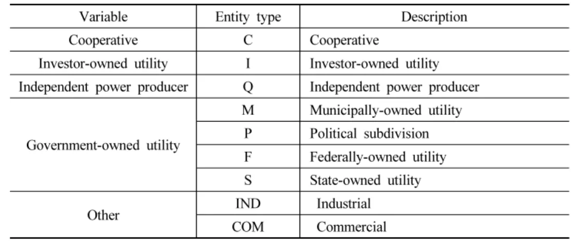
Data on nameplate capacity by technology type and ownership structure is collected from EIA 860. Table 2 shows the prime mover codes that are reported in EIA 860 for each generator. I aggregate the generator nameplate capacity by the prime mover code at the firm given year, then aggregate the prime mover codes into four technology types to calculate nameplate capacity of plants by the technology type in the firm. Finally, Table 3 shows the nine types of ownership available in EIA 860 that best describes the firms that owns and operates the plants. Industrial and commercial firms are not considered in the paper as their principal business is not electricity generation. Since there are only a few independent power producers or government-owned utilities that are reported in both Form 1 and EIA 860, cooperatives and investor-owned utilities are the only ownership structures that are considered in this paper.
<Table 3> Ownership type in EIA 860
Variable Entity type Description
Cooperative C Cooperative
Investor-owned utility I Investor-owned utility Independent power producer Q Independent power producer
Government-owned utility
M Municipally-owned utility P Political subdivision F Federally-owned utility S State-owned utility
Other IND Industrial
COM Commercial
2. Summary Statistics
Table 4 presents summary statistics of the variables collected from Form 1 distinguished by the ownership structure. Each ownership structure is again separated
into those with and without having large plants. Table 4 shows considerable variation across the groups. Cooperatives even having large plants are a lot smaller than IOUs without large plants, measured by total assets, net income, operating and electric revenues, or total mwh sold. For example, the value of total assets of cooperatives with large plants is $789 million on average, while that of IOUs with and without large plants is $3707 and $5636 million, respectively. Most part of operating revenues is earned from electric revenues for both types of ownership, but IOUs are more diversified, in a sense that the IOUs report on average about 10% of revenues from other than electricity. Both cooperatives and investor-owned utilities report positive sales of electricity to ultimate
<Table 4> Descriptive statistics of rm performances by ownership
Ownership
Cooperative IOU
No large plant Large plant No large plant Large plant Total Assets ($ mil) 203 (221) 789 (539) 3707 (6337) 5636 (6420) Shareholder Equity ($ mil) 60 (68) 172 (113) 1137 (1893) 1764 (2136) Long-Term Debt ($ mil) 112 (136) 450 (321) 1148 (1869) 1633 (1699) Interest Charges ($ mil) 5 (7) 29 (17) 67 (122) 95 (98) Dividends ($ mil) 0.85 (2.49) 0 (0) 69 (144) 114 (176) Net Income (after tax, $ mil) 13 (15) 34 (22) 212 (414) 343 (433) Net Income (before tax, $ mil) 13 (15) 34 (22) 243 (478) 378 (490) Operating Revenues ($ mil) 121 (128) 446 (256) 1349 (2219) 2076 (2159) Electric Revenues ($ mil) 116 (127) 446 (256) 1189 (1863) 1896 (2033) Electric Expenses ($ mil) 97 (115) 382 (228) 790 (1224) 1282 (1361) Total mWh sold (mWh mil) 1.6 (1.9) 7.9 (3.5) 15.6 (24.3) 53.3 (462) Portion of Sales for Resale 0.38 (0.42) 0.99 (0.002) 0.21 (0.33) 0.29 (0.27) Portion of Sales to Ultimate Consumers 0.61 (0.42) 0.001 (0.002) 0.78 (0.33) 0.70 (0.27) Portion of Electricity Purchases 0.85 (0.30) 0.58 (0.30) 0.74 (0.35) 0.34 (0.24) Portion of Electricity Generation 0.15 (0.30) 0.41 (0.30) 0.24 (0.35) 0.65 (0.24)
Number of Firms 36 6 102 94
Number of Observations 138 67 1053 1094
Notes: Standard deviations are in parentheses.
consumers and sales for resale, suggesting vertically integrated structures.
6)
Although Table 4 shows virtually all transactions are sales for resale for the large cooperatives, these cooperatives are vertically integrated with their member distribution cooperatives through long-term power purchases contracts. Both cooperatives and investor-owned6) Sales for resale means the transactions in wholesale electricity markets. Sales to ultimate consumers means the retail side of electricity, ranging from the service for a large industrial facility to small businesses and to individual households.
<Table 5> Firm performances by ownership
Ownership Cooperative IOU
No large plant Large plant No large plant Large plant Portion of Long-Term Debt in Total Assets 0.46
(0.20)
0.57 (0.11)
0.25 (0.10)
0.29 (0.08) Portion of Equity in Total Assets 0.35
(0.18)
0.23 (0.10)
0.36 (0.18)
0.30 (0.09) Portion of Liabilities in Total Assets 0.64
(0.18)
0.76 (0.10)
0.63 (0.18)
0.69 (0.09)
Cost of Debt 0.03
(0.01)
0.05 (0.01)
0.02 (0.01)
0.02 (0.01)
Cost of Equity 0.007
(0.02)
0 (0)
0.06 (0.08)
0.06 (0.05) Return on Assets (after tax) 0.06
(0.04)
0.05 (0.03)
0.06 (0.04)
0.06 (0.03) Return on Assets (before tax) 0.06
(0.04)
0.05 (0.03)
0.07 (0.06)
0.06 (0.04) Return on Equity (after tax) 0.45
(1.87)
0.22 (0.11)
0.18 (0.70)
0.29 (0.75) Return on Equity (before tax) 0.45
(1.87)
0.22 (0.11)
0.22 (0.75)
0.32 (0.81)
Cost of Capital 0.02
(0.01)
0.04 (0.01)
0.03 (0.06)
0.03 (0.04)
Capacity Factor 0.27
(0.24)
0.48 (0.36)
0.31 (0.24)
0.45 (0.16)
Number of Firms 36 6 102 94
Number of Observations 138 67 1053 1094
Notes: Standard deviations are in parentheses.
utilities without large plants heavily rely on purchased electricity. Specifically, cooperatives without large plants purchase 85% of the total electricity sales on average, while investor-owned utilities without large plants buy 74% of the total electricity sales from other firms. Although the portion of purchased electricity is reduced, cooperatives with large plants still purchase more than half of the total electricity in wholesale markets. On average, investor-owned utilities with large plants generate about two-thirds of the total electricity.
The variables presented in Table 4 are used to calculate performance outcomes shown in Table 5. I calculate cost of debt (COD) by dividing interest charges by total liabilities, which is equal to total assets net of shareholder equity. Cost of equity (COE) is computed by dividing dividends declared by shareholder equity. The measure of cost of capital is the weighted average of interest charges and dividends multiplied by the proportional weight of debt and equity in total assets, respectively, then taking the sum of the terms.
Specifically, weighted average cost of capital (WACC) is calculated as
(1)where E denotes shareholder equity, A total assets, D dividends, L total liabilities, I interest charges, t tax rate. Therefore, WACC reflects a firm’s cost of capital that the firm is expected to pay on average to finance its assets. To measure profitability, return on assets (ROA) is calculated as before and after taxes net income divided by total assets at the beginning of year. Similarly, return on equity (ROE) is before and after taxes net income divided by shareholder equity at the beginning of year.
Finally, capacity factor is calculated as the ratio of electricity produced in plants owned by firm over year to the potential output if it were possible for the firm to operate its plants at full nameplate capacity continuously over the year. Therefore, capacity factor measures an aggregated efficiency of plants in a firm conditional on
operation.
7)
Table 5 shows that cooperatives more rely on long-term debt than IOUs, as indicated by higher portion of long-term debt in total assets. While long-term debt accounts for about half of total assets for cooperatives, investor-owned utilities finance less than one-third of their total assets from long-term debt. Interestingly, the mix of equity and liabilities is not very different for small cooperatives compared to small or large investor-owned utilities, but large cooperatives distinctively rely on liabilities than equity. This suggests that cooperatives are subject to more stringent constraints to expand firm size as they have limited access to external equity capital. Moreover, the fact that long-term debt accounts for higher portion of liabilities for cooperatives suggests that investor-owned utilities tend to borrow to fund its current operations, such as purchasing inputs, while cooperatives take on long-term debt in order to acquire capital, such as plants. This is consistent with the cost of debt significantly increasing for cooperatives, especially the ones having large plants. While IOUs on average declare about 6% of equity as dividends, cooperatives have significantly lower cost of equity, about 0.7% and 0%, for cooperatives without and with large plants, respectively. For small cooperatives, higher cost of debt is compensated with the lower cost of equity, leading to insignificantly different cost of capital. However, even zero cost of equity does not fully offset higher cost of debt for large cooperatives, yielding higher cost of capital than other groups. IOUs show higher return on assets than cooperatives before income taxes, but have about the same return on assets after income taxes. This is because cooperatives are exempt from federal income taxation as far as 85% or more of their income is collected from the members. Although return on equity seems higher in cooperatives compared with investor-owned utilities, it also shows higher standard deviations than other performance measures. Finally, capacity factor is higher for large
7) As Davis and Wolfram (2012) discussed, the capacity factor might not be an appropriate measure of
efficiency if some firms excercise market power. For example, operating a portfolio of generating
plants, a firm might nd it profitable to withhold capacity from some plants whose marginal costs are
closer to the market clearing price.
plant groups for both cooperatives and IOUs, but it does not confirm as it does not take into account that the capacity factor varies greatly across fuel and plant types. In the estimation the specications control for observable characteristics of firms including the mix of plant technologies.
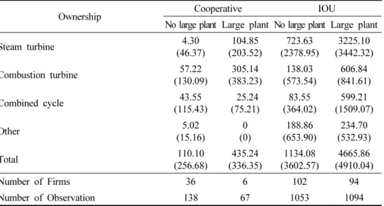
Table 6 presents the controls on plant type and capacity obtained from EIA 860. Table 6 shows an interesting distinction between cooperatives and investor-owned utilities.
Investor-owned utilities use steam turbine as the dominant mode of electricity generation, while for cooperatives combustion turbine is the most important mode. This reflects some systematic differences in operating decisions across the ownership structures, as the selection of plant technologies and capacity is related with the firm’s decision on the scale of generation and the trade-off between construction costs and operating costs. Steam turbine uses coal or nuclear as a fuel to create steam and have a relatively low thermal efficiency, but its fuel costs is low, so steam turbine is used to meet base demand by supplying electricity nearly continuously and its relatively high construction costs are spread over continuous operation. In general, capacity of steam
<Table 6> Plant type and capacity by ownership from EIA 860
Ownership Cooperative IOU
No large plant Large plant No large plant Large plant
Steam turbine 4.30
(46.37)
104.85 (203.52)
723.63 (2378.95)
3225.10 (3442.32)
Combustion turbine 57.22
(130.09)
305.14 (383.23)
138.03 (573.54)
606.84 (841.61)
Combined cycle 43.55
(115.43)
25.24 (75.21)
83.55 (364.02)
599.21 (1509.07)
Other 5.02
(15.16)
0 (0)
188.86 (653.90)
234.70 (532.93)
Total 110.10
(256.68)
435.24 (336.35)
1134.08 (3602.57)
4665.86 (4910.04)
Number of Firms 36 6 102 94
Number of Observation 138 67 1053 1094
Notes: Standard deviations are in parentheses.
turbine plants is greater than that of other technologies. On the other hand, combustion turbine generates electricity by burning natural gas with higher thermal efficiency than that of steam turbine. Combustion turbine requires higher operating costs, especially fuel, which is a trade-off for lower construction costs. Typical size of combustion turbine is smaller than that of steam turbine. The fact that cooperatives have combustion turbine as the dominant mode of generation suggests that the cooperatives generate electricity during the periods of peak demand, while purchase electricity in wholesale markets during off-peak hours, when electricity prices are low. Both cooperatives and investor-owned utilities have some capacity of combined cycle plants. Investor-owned utilities also employ other types of technology, especially renewable energy plants.
III. Empirical Model
1. Differences between Cooperatives and IOUs
I first use the data to see if there are any systematic differences between cooperatives and IOUs that would lead to different performance outcomes measured from accounting information. I compare the firms along several dimensions: cost of debt (COD), cost of capital (WACC), return on assets after and before income taxes (ROA-A, ROA-B), return on equity after and before income taxes (ROE-A, ROE-B), and capacity factor (CU). Following the standard difference-in-difference specifications, the estimating equations have the form:
Ownership
Large Plant
Ownership
‧ Large Plant
(2)where
refers to the performance measures of firm i in year t, Ownershipi is a dummy equal to 1 firm i is a cooperative and zero otherwise. Similarly, Large Plantit is a dummy that turns on if firm i has a large plant in year t. Xit is a vector of firm level controlsincluding portion of electricity sales for resale and portion of electricity purchases in Table 4, and a set of nameplate capacity of plants owned by the firm distinguished by technology type reported in Table 6. The year fixed effects,
, measures industry-level shifts over time, such as sector-level technology shocks or fuel price fiuctuations. Finally, potential spatial heterogeneity in which firms operate, such as regulatory environment, is controlled using time-invariant region effects
.8)
it is an unanticipated i.i.d. shocks to the performance outcomes including the measurement error. Therefore, I look at performance differences between the two ownership types by comparing firms within a region controlling for the industry-wide shocks (
) and firm characteristics (
it). The specification (2) allows us to interpret coefficients to those in standard difference-in-difference estimations, where the coefficient
indicates the changes in performance outcomes of large cooperatives relative to those of large investor-owned utilities conditional on the decisions of ownership and large plant investments. Estimates have robust standard errors clustered at the regional level.I note that the decisions on ownership structure and large plant investments are not exogenous. However, in the data the ownership structure of the firms was determined prior to the sample period, and given that the investments in large plants are long-term decisions, the error term in (2) is not correlated with the ownership and large plant indicators in a given year. Alternatively, the identification in (2) in part rely on the assumption that the causal effect of large plant investments create a discrete change in the performance outcomes around the event, whereas after controlling for observable characteristics of the firms, any performance trends that might lead to the selection would be common to the firms in a given regional market and a year so that partialled out in the fixed effect specications, or gradual enough to be distinguished from the discrete direct effects (Braguinsky et al., 2015).
8) The regions are as defined by the North American Electric Reliability Council (NERC)
2. The Estimation of Cost Function
As I will discuss in the next section, the analysis of performance outcomes in (2) suggests that cooperatives and investor-owned utilities face significantly different cost structures to finance their assets. The purpose of this section is to recover the fixed and the marginal costs of operation across the firms. By comparing the shape of the cost function across the ownership structures I can confirm the systematic differences between cooperatives and investor-owned utilities.
Consider the following model of cost minimization. To generate electricity output, denoted by
, a firm needs to combine three input factors: labor (L), fuel and nonfuel materials (M), and power plants (K). The firm specific productivity (
) is known to the firm but not observed by the researcher. For firm i in year t, I specify the production function asQgit = Q (Lit, Mit, Kit,
it) (3)Let Q ≡ Qg + Qpdenote the total electricity output sold by firm, where Qpdenotes the purchased electricity. Given the production function in (3), the conditional cost function from the cost minimization is defined by
min
subj ect to
≡ P
it
(4)
where Pit ≡(Plit, Pmit, Ppit) denotes the vector of input prices. The dependent variable Cit
measures the total costs of electric operation and maintanence. In equation (4), firm i chooses the cost minimizing amount of generated (Qgit) and purchased (Qpit) electricity given the production technology and the total electricity demand (Qit) faced by the firm.
Equation (4) is a conditional cost function in the sense that it includes the power plant
capacity, the total electricity output, and the productivity.
In the estimation of (4), an issue is the potential for simultaneity in the relationship between Qit and Cit. This would arise if firms adjusted their output to accommodate the productivity shocks (
it) which is also correlated with Cit. I accommodate the endogeneity of output (Qit) by instrumenting for it with the mean of deviations of other firms’ wholesale electricity prices from the regional average wholesale electricity price that are in the same region with firm i, denoted by ∆
, where -i and s index all other firms than firm i and regional wholesale market, respectively, which will be further explained below. It will be a valid instrument if, for firm i in region s in period t, the two conditions hold. First, ∆
need be correlated with Qit. This will be true if changes in
, i.e., changes in other firms wholesale electricity prices that are in the samewholesale market s, are correlated with regional electricity demand that is also correlated with Qit. Second,
∆
need be uncorrelated with the error term in the cost function of firm i in year t. To investigate this, let us model the wholesale price for firm i in region s in year t as
(5)where
is the wholesale electricity price received by firm i in region s in year t,
is the marginal cost of electricity generation, and d (
) is a demand shock for firm i in region s in year t. Equation (5) is a familiar equation where price is equal to marginal cost, but potentially deviate from the marginal cost influenced by demand- side factors. I can decompose equation (5) into the regional mean (
) that is common to all firms in region s in year t and the deviation from this mean that is firm-specific.
≡
∆
∆
≡
∆
(6)
where I use the mean of
∆
for all firms but firm i in the same region s in period t, ∆
, to instrument Qit. The idea is that after eliminating region-specific time-varying components that are common to all firms in a region, the price variations across the firms in region s in year t are driven by firm-specific shifters, which provide an instrumental variable that is correlated with Qist through the regional electricity demand but uncorrelated with the error term in the cost function Cit given that∆
is induced by either marginal cost or demand shocks that are specific to individual firms
.In the estimation, I specify the log of the cost function in (4) as
‧
Ownershipi +
Ownershipi +
(7)
where the small letters indicate the log of the variables. Since the productivity
it is unobservable, equation (7) includes the two error terms,
it and
it, where
it represents an i.i.d. error term in the estimation. Therefore, the coefficients in (7) are identified in the second stage if ∆
is uncorrelated with the unobserved productivity
it but correlated with
it. I also control for industry-wide shocks using year fixed effects,
. By including the ownership dummy, the specification in (7) allows that the returns to scale can be different across the ownership structures. Finally, by the duality theory, the cost function is homogenous of degree one in input prices. In equation (7), this is imposed by normalizing the material and purchased power prices (
and
) by the labor price (
), the log of which are represented by
and
, respectively.IV. Results
In this section, I start with the discussion of the performance outcome regressions. I then proceed to present the cost function estimation results where I quantify the marginal cost of operation across the ownership structures.
1. Differences in Performance Outcomes
Table 7 shows the results from the estimation of (2) for various performance outcome variables. In the column (1), the result for the cost of debt regression indicates that comparing between small cooperatives and small investor-owned utilities, small cooperatives have higher cost of debt than small investor-owned utilities by 1 percent.
Having large plants increases the cost of debt for investor-owned utilities by 0.3 percent.
Relative to large investor-owned utilities, cooperatives with large plants have higher cost of debt by 1.6 percent, suggesting that investing in large plants is more costly for cooperatives. The estimates are statistically signicant at 5 percent or stricter.
In the weighted average cost of debt and equity regression, in the column (2), the estimate for the interaction coefficient
is positive and statistically significant at 1 percent. Even with the higher cost of debt partly offset by zero dividends, the weighted average cost of capital is still higher for large cooperatives than those counterparts by 1.5 percent. However, for small cooperatives the insignificant estimate
indicates that the lower cost of equity effectively compensates the higher cost of debt, resulting in statistically indifferent weighted average cost of debt and equity.The columns (3) to (6) present the regression results of the profitability outcomes, return on assets and return on equity. I do not find systematic differences between cooperatives and investor-owned utilities in these outcome variables. On the other hand, the coefficients for large plant are significant at 10 percent in the columns (3) and (4), by 1.3 and 1.8 percent, using net incomes after and before income taxes, respectively, which
<Table 7> Comparison of rm performances between Cooperatives and IOUs Dependent variable
(1) (2) (3) (4) (5) (6) (7)
Coefficient on COD WACC ROA-A ROA-B ROE-A ROE-B CU Cooperative 0.01**
(0.003)
-0.003 (0.003)
0.005 (0.007)
-0.006 (0.009)
0.35 (0.32)
0.32 (0.32)
0.01 (0.07) Large plant 0.003**
(0.001)
-0.011 (0.006)
-0.013*
(0.007)
-0.018*
(0.008)
0.11 (0.07)
0.11 (0.08)
0.05 (0.06) Cooperative×
Large plant
0.016**
(0.007)
0.015**
(0.003)
-0.016 (0.01)
-0.01 (0.01)
-0.74 (0.40)
-0.78 (0.43)
0.08 (0.17) Firm
controls Portion of
sales for resale
-0.008**
(0.002)
-0.006 (0.007)
1.01 (1.01)
0.01 (0.01)
0.37 (0.33)
0.42 (0.36)
0.09 (0.08) Portion of
electricity purchases
-0.002 (0.003)
-0.02**
(0.008)
-0.01 (0.008)
-0.02*
(0.009)
-0.11 (0.13)
-0.10 (0.13)
-0.41**
(0.06) Steam
turbine
-0.61**
(0.08)
-0.28 (0.22)
0.63 (0.45)
0.44 (0.50)
-2.22 (9.20)
-2.81 (9.37)
-4.05 (5.89) Combustion
turbine
0.61 (0.34)
-1.48 (1.09)
0.41 (1.06)
2.03 (1.23)
-41.01 (39.65)
-36.57 (41.68)
-42.18 (25.88) Combined
cycle
-0.41**
(0.16)
0.0005 (1.17)
-0.97**
(0.23)
-1.49**
(0.27)
-0.35 (9.61)
-2.42 (10.45)
-7.86 (7.75)
Other 0.28
(0.88)
1.32 (1.58)
-1.23 (2.50)
-1.55 (3.65)
45.98**
(19.78)
53.60*
(23.73)
45.88*
(24.40) Region fixed
effects Yes Yes Yes Yes Yes Yes Yes
Year fixed
effects Yes Yes Yes Yes Yes Yes Yes
F-statistic 10.73** 154.84** 813.50** 83.73** 1504.68** 49.29** 6680.13**
Observations 2149 2149 2135 2135 2135 2135 1325
R
20.29 0.04 0.09 0.11 0.06 0.07 0.48
Notes: Robust standard errors are clustered at the region in parentheses. Dependent variables are the performance outcomes presented in Table 5: COD is cost of debt, WACC cost of capital, ROA-A and ROA-B return on assets after and before income taxes, respectively, ROE-A and ROE-B return on equity after and before income taxes, respectively, and CU capacity factor.
** Signicant at 5 percent or stricter.
* Signicant at 10 percent.
indicate the differences in return on assets between small and large investor-owned utilities. The lower return on assets implies that relative to small investor-owned utilities, large investor-owned utilities generate lower net income given level of assets, or have excessive assets to generate given level of net income. Although it is not the scope of this paper, this is consistent with the hypothesis suggested by Averch and Johnson (1962) where regulated investor-owned utilities overinvest in capital under the cost of service regulation, as new investment in capital becomes part of the rate of return calculation allowed to investor-owned utilities. The column (7) presents the comparison of capacity utilization across the ownership structures. I do not find systematic differences between the two groups. Finally, Table 7 also shows that the firm control variables(
) are important determinants of the firm performance outcomes and well capture the individual heterogeneity. For example, in the column (1), an increase in the portion of sales for resale, i.e., the portion of sales in wholesale markets, decreases the cost of debt.The column (7) indicates that an increase in the portion of electricity purchases decreases the capacity utilization. In all the specifications, F-statistics reject the null that all of the region and year dummy variables are zero, suggesting that the fixed effects control some heterogeneity at the region given a year.
2. Differences in the Cost of Operation
The analysis in Section 4.1 revealed some systematic differences between cooperatives and investor-owned utilities. In particular, I saw that cooperatives operate under conditions of more constrained access to capital associated with higher cost of debt and limited availability of external equity. However, I did not find cooperatives are necessarily less profitable or efficient than investor-owned utilities. In this section I proceed to investigate whether there are any differences in the cost structure of operation across the ownership forms, and recover the marginal costs of operation.
Table 8 presents the results of the OLS estimation of the cost function in (7). As I note
that about one-third of the firms in the data does not own power plants, I estimate the separate cost function for the firms that own generating capacity and those that do not own generating capacity. Table 8 shows the coefficient of
is 0.76 and 0.90 for plant owners and non-plant owners, respectively, suggesting positive scale economies for both plant and non-plant owners. The interaction term between
and Ownershipi is not significant in both columns, nor is Ownershipi, implying that both the marginal and fixed cost of operation are not different across the ownership structures. However, as I discussed, if there is bias due to the correlation between
and
, the coefficients are imprecisely estimated.<Table 8> OLS estimation of the cost function
Plant No plant
Coefficient on (1) (2)
0.76**
(0.14)
0.90**
(0.03)
‧ Ownership
i0.03
(0.08)
-0.007 (0.03)
Ownership
i-0.12
(0.19)
-0.06 (0.11)
0.13
(0.11)
0.54**
(0.14)
0.39**
(0.12)
0.15 (0.12)
0.06
(0.07)
Constant 0.72**
(0.25)
0.84**
(0.08)
Year fixed effects Yes Yes
Region fixed effects Yes Yes
Observations 1364 651
R
20.92 0.94
Notes: Robust standard errors are in parentheses.
** Signicant at 5 percent or stricter.
* Signicant at 10 percent.
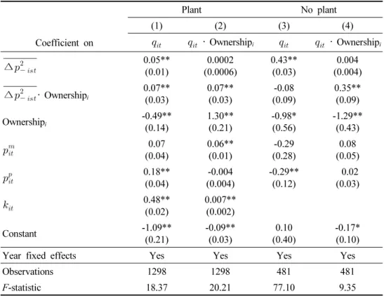
Table 9 shows the results of the first stage regression using
∆
as the instrument.The instrument is a strong predictor of the electricity output. For example, in the column (1), for every 10 percent increase in the mean of the competing firms’ deviation from the regional wholesale price, electricity output for firm i increases by 0.5% and 1.2% for investor-owned utilities and cooperatives, respectively, which are statistically significant at 5 percent or stricter. In addition, the first stage F-statistics are large, suggesting that the instrument is not weak.
<Table 9> First stage estimation of the cost function
Plant No plant
(1) (2) (3) (4)
Coefficient on
‧ Ownership
i
‧ Ownership
i ∆
0.05**
(0.01)
0.0002 (0.0006)
0.43**
(0.03)
0.004 (0.004)
∆
‧ Ownership
i0.07**
(0.03)
0.07**
(0.03)
-0.08 (0.09)
0.35**
(0.09)
Ownership
i-0.49**
(0.14)
1.30**
(0.21)
-0.98*
(0.56)
-1.29**
(0.43)
0.07
(0.04)
0.06**
(0.01)
-0.29 (0.28)
0.08 (0.05)
0.18**
(0.04)
-0.004 (0.004)
-0.29**
(0.12)
0.02 (0.03)
0.48**
(0.02)
0.007**
(0.002)
Constant -1.09**
(0.21)
-0.09**
(0.03)
0.10 (0.40)
-0.17*
(0.10)
Year fixed effects Yes Yes Yes Yes
Observations 1298 1298 481 481
F-statistic 18.37 20.21 77.10 9.35
Notes: Robust standard errors are in parentheses.
** Signicant at 5 percent or stricter.
* Signicant at 10 percent.
The second stage results of the cost function estimation are presented in Table 10. It is interesting to note that the coefficient of
moves downward, while that of the interaction term
‧ Ownershipi moves upward in both columns, suggesting that bias induced by the simultaneity between
and
has different directions for cooperatives and investor-owned utilities. The upward bias would arise if the correlation between
and
has the same sign with the correlation between
and
in equation (7). In contrast, the downward bias would arise if the two correlations have the opposite signs.Let us assume that there is a positive simultaneity between
and
in both types of ownership structure, i.e., more productive firms sell more electricity, either by producing<Table 10> Second stage estimation of the cost function
Plant No plant
Coefficient on (1) (2)
0.28*
(0.16)
0.76**
(0.76)
‧ Ownership
i0.83**
(0.38)
-0.07 (0.07)
Ownership
i-1.62**
(0.68)
-0.17*
(0.09)
0.15**
(0.04)
0.54**
(0.09)
0.48**
(0.08)
0.18 (0.11)
0.28**
(0.08)
Constant 0.29
(0.18)
1.04**
(0.12)
Year fixed effects Yes Yes
Observations 1298 481
F-statistic 107.79 154.07
Notes: Robust standard errors are in parentheses.
** Signicant at 5 percent or stricter.
* Signicant at 10 percent.
in their plants or by purchasing from wholesale markets. Since the output coefficient moves downward for investor-owned utilities in Table 10, I expect that there is a positive relationship between
and
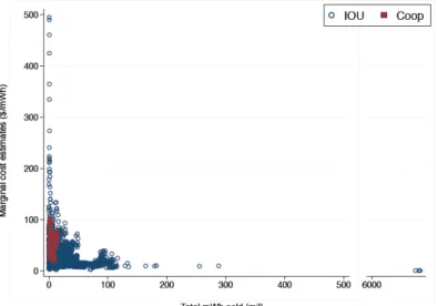
, i.e., more productive firms incur higher cost of operation holding output at constant. This is possible if more productive firms sell more outputs but there exists inefficiency associated with cost of operation in the firms, e.g., suboptimal allocation of inputs, which lead to increased cost of operation. Or, efficiency could be negatively affected if there was market power exercised by some firms in the market, which would typically be large firms.As Joskow (1997) discussed, this result may support that very large electric companies are not neccesary to exploit the economies of scale available in the industry. The cost efficiency of operation would rather depend on the ability to coordinate power plants and transmission network dispersed over geographic areas. The marginal cost estimates that will be discussed below also show that the marginal cost of operation is virtually at once the output level reaches a certain point. In contrast to investor-owned utilities, I find the coefficient moves upward for cooperatives in the IV regression, i.e., the estimate is biased downward in the OLS estimation. Thus I expect that there is a negative relationship between
and
, suggesting that more productive cooperatives incur lower costs of operation holding the output levels at constant. Note that it is not inconsistent with the results in columns (3) and (4) of Table 7, where I found large investor-owned utilities have lower ratio of net income in total assets than small investor-owned utilities.The column (1) in Table 10 also suggests that the fixed cost of operation, indicated by different intercepts across the ownership structures, Ownershipi, is lower for cooperatives, whereas the marginal cost of operation
Ownershipi more sharply increases with the output for cooperatives relative to investor-owned utilities. In contrast, in the column (2) where I estimate the cost function of non-plant owners, I still find the fixed cost of operation is lower for cooperatives, but the marginal cost structureis not different between the two ownership types. In both cases, the results show that the electric power industry is characterized by substantial positive scale economies with the magnitude of 0.28 and 0.76 for plant and non-plant owners, respectively, except that I cannot reject the constant returns to scale for cooperatives with power plants. Figure 1 evaluates the cost function using the IV estimates over a range of electricity outputs for each of ownership structures while holding other variables at the sample means. Each of the dots in Figure 1 represents the mean of the total costs of operation and the electricity output in each group. The scale economies persist for large investor-owned utilities.
Moreover, the sample mean of large investor-owned utilities operate in the fiat area of the cost curve.