Convergent association between socioeconomic status and the blood concentrations of mercury, lead, and cadmium in the Korean
adult population: based on the sixth Korea National Health and Nutritional Examination Surveys (KNHANES 2013-2015)
Junghyun Kim, Youngtae Cho*
Department of Public Health, Graduate School of Public Health, Seoul National University
한국성인의 사회경제적수준과 혈중 중금속 농도의 융합적 분석
김정현, 조영태*
서울대학교 보건대학원 보건학과
Abstract The purpose of this study was to investigate the association between socioeconomic status and blood heavy metal concentration in Korean adult population using the Korea National Health and Nutritional Examination Survey(KNHANES 2013-2015). Multiple logistic regression analysis was used to determine the association between socioeconomic status and the blood heavy metal concentration.
Positive association was found between education and income level and blood concentration of mercury while those of lead and cadmium were negatively associated education and income level in Korean adult population (P for trend <0.001). At the point of an increase in the prevalence of heavy metal concentrations in the blood, a national public health policy will be needed to address the inequity of health due to socioeconomic factors.
Key Words : Convergence, Mercury, Lead, Cadmium, Heavy metal, SES
요 약 본 연구는 사회경제적 상태의 지표인 교육수준 및 소득수준과 수은, 납, 카드뮴의 혈중 중금속 농도간의 관련성 을 살펴보고자 하였다. 국민건강영양조사 2013-2015년 자료를 이용하여 성별에 따른 사회경제적상태와 혈중 중금속 농도간의 관련성을 분석하기 위해 로지스틱회귀분석을 실시하였다. 분석결과 한국성인의 교육과 소득수준이 높을수록 혈중 수은의 농도는 증가하는 경향이 나타났고, 혈중 납과 카드뮴의 농도는 감소하는 경향을 보였다 (P for trend
<0.001). 혈중 중금속 농도의 유병률이 증가하고 있는 시점에서 사회경제적수준에 따른 건강불평등을 해결하기 위한 국가차원의 공중보건학적 정책이 필요할 것으로 사료된다.
주제어 : 융합, 수은, 납, 카드뮴, 중금속, 사회경제적수준
*Corresponding Author : Youngtae Cho([email protected]) Received January 30, 2019
Accepted March 20, 2019 Revised February 27, 2019
Published March 28, 2019
1. Introduction
Recently, heavy metal contamination in the body has become a serious hazards to health. In Korea, environmental diseases are increasing with the industrial development, mass production of chemicals including heavy metals, and air pollution from the increased traffic. Changes in lifestyle cause higher incidence and mortality of chronic diseases such as cardiovascular disease[1-4].
Increasing the heavy metal concentration in the body causes various diseases. Heavy metals absorbed by the body through various ways such as digestive organs and circulatory organs are mostly excreted. However, it is the portion that are deposited in the tissues and blood, that causes various diseases including hormonal metabolic disorders, high blood pressure, diabetes, cancer, osteoporosis, and kidney disease[5-11]. Mercury is used in many parts of the industry and builds up in the body through the ecosystem food chain. In particular, the mercury concentration in Asian blood is found to be two to three times higher than that of Americans, which was highly associated with the consumption of fish[12,13]
and drinking alcohol[14]. Lead and Cadmium that builds up in nerves, kidneys, endocrine systems, genitals and in other areas of the body cause hormonal metabolic disorders, and deposition in the cardiovascular system cause thrombosis and high blood pressure[15]. In particular, blood lead concentration was high among smokers[16] and alcohol drinkers[17-19], and it has been found that air pollution form traffic[20] affects cadmium exposure in children aged 11 to 13 [12,14]. The increase in blood heavy metal concentration is mainly influenced by not only genetics but also environmental factors, and rapid changes in lifestyle are increasing the importance of the environmental factors[6,20].
Research on the effects of socioeconomic conditions on blood heavy metals concentration has been increasing recently[21-24]. Social and
economic factors are known to be highly associated with diet, exercise, and health behaviors that affect the concentration of heavy metals in blood[25-28]. Higher the concentration of lead and cadmium in the blood was estimated for people in low socioeconomic status due to poor lifestyle such as smoking and drinking.
Many studies have reported that lower socioeconomic level was associated with higher the level of lead and cadmium in the blood, and that higher socioeconomic level was associated with higher blood concentration of mercury[21,22]. A 34 year tracking survey conducted in Alameda County in the U.S. also reported that the lower the socioeconomic status, especially lower the level of education, the higher the blood lead and cadmium concentration[21]. A study conducted in the U.S. showed that blood lead concentration of African American in low education level was higher than American's in high education level, and low-income people's blood lead concentration was higher than high-income people[23]. However, most of the studies involved are mainly from the West, and studies focusing on social and economic conditions for Koreans are lacking.
The purpose of this study was to investigate the association between education and income levels which are the indicators of socioeconomic status (SES) to blood heavy metal concentration such as mercury, lead and cadmium using Korea National Health and Nutritional Examination Surveys (KNHANES).
2. Materials and Methods
2.1 Study ParticipantsThis study was based upon the data obtained in the first, second and third year of Korea National Health and Nutritional Examination Survey (KNHANES) Ⅵ (2013-2015). KNHANES which examined a health examination, a health interview, and a nutrition survey is conducted
annually, using the stratified multistage cluster sampling method that drew on a representative sample of the non-institutionalized civilian population in South Korea. We analyzed the data of (n=7,999) participants over aged 20 years old who completed the nutrition survey and the health examination survey, including blood metal measurements. All the participants in the survey received informed consent.
2.2 Demographic, anthropometric variables and socioeconomic status (SES)
We included age, gender, residence area(urban), physical exercise, alcohol drinking, smoking status as demographic variables and education level, and household monthly income level as socioeconomic indicators during the health interview survey and Waist circumference (WC), Body mass index (BMI) as anthropometric variables. Residence area was divided into two categories; Rural or urban. Rurality of residence is determined by health interview survey.
Physical exercise was divided into two groups;
non-exercise group, regular exercise group.
Regular exercise group means those who exercise more than three times a week and more than 20 minutes for one time. Based on the frequency of monthly alcohol drinking, alcohol intake was classified into three groups;
non-drinkers, mild to moderate drinkers, heavy drinkers. Those who drank more than once a month were defined as drinkers and those who drank more than three drinks a day were defined as heavy drinkers. Smoking status was categorized into three groups; non-smokers, ex-smokers, current-smokers. Those who smoked more than five packs for a lifetime defined as smokers. We distinguished ex-smokers from current-smokers based on the present smoking status. Education level was classified into four groups; Elementary school, middle school, high school, and college and higher. And monthly income level was divided into four groups
according to quartiles: low, middle low, middle high, high. Waist circumference (WC) was measured at the narrowest point between the lower border of the rib cage and the iliac crest.
Body mass index (BMI) was calculated using the following formula: weight (kg) / height2 (m2).
2.3 Measurement of Mercury, Lead, and Cadmium
To assess levels of heavy metals in whole blood, 3ml blood samples were obtained from the anticubital vein after the participants have been fastened for eight or more hours to determine the blood level of mercury (Hg), lead (Pb), and cadmium (Cd). Blood samples were processed appropriately, then immediately refrigerated, and transported by cold storage to the Central Testing Institute in Seoul, Korea. Blood samples were analyzed within 24 hours after transportation.
Blood lead and cadmium were measured by graphite-furnace atomic absorption spectrometry with Zeeman background correction(Perkin Elmer A Analyst 600; Perkin Elmer, Turku, Finland). Blood total mercury levels were measured using a gold amalgam collection method with a DMA 80 (Milestone, Bergamo, Italy). For internal quality assurance and control, commercial reference materials were used (Lyphochek Whole Blood Metals Control; Bio-Rad, Hercules, CA, USA). The coefficients of variation were within 0.95–4.82 %, 2.65–6.50 %, and 1.59–4.86 % for blood cadmium, lead, and mercury, respectively in four reference samples. As part of external quality assurance and control, the institute passed both the German External Quality Assessment Scheme operated by Friedrich-Alexander University and the Quality Assurance Program operated by the Korea Occupational Safety and Health Agency.
The method detection limits for blood cadmium, lead, and mercury in the present study were 0.056 μg/l, 0.12 μg/dl, and 0.158 μg/l, respectively. No sample for blood cadmium, lead, or mercury was the below detection limits.
2.4 Statistical analysis
All analyses were performed using the SAS (Version 9.2; SAS Institute, Cary, NC, USA). One way analysis of variance (ANOVA) was used to investigate the differences in demographic variables according to household income and education levels. A multiple logistic regression analysis was used to confirm the odds ratios (ORs) and 95% confidence intervals (CIs) for the blood level of heavy metal according to each demographic variable. Two-sided P-value <0.05 was considered statistically significant.
3. Result and discussion
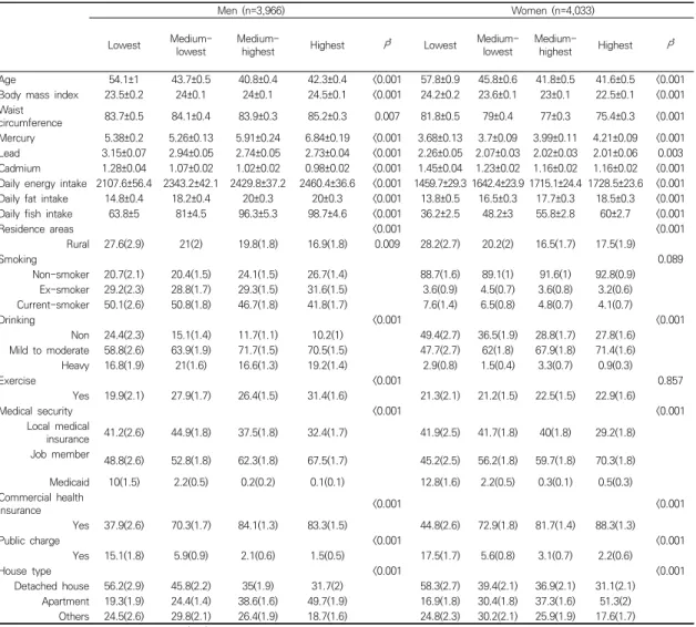
The general characteristics of study participants according to gender are shown in Table 1. The participants consisted of 7,999 men (49.6%) and 4,033 (50.4%). The average age of men was 44 years old and women was 46 years old. The means of blood mercury, lead, and cadmium concentration for men were 5.93 μg/l, 2.85μg/dl, and 1.06μg/l, respectively and those for women were in 3.91μg/l, 2.08 μg/dl, and 1.24 μg/l, respectively. Men smoked much more and had a higher level of alcohol consumption than women, despite the fact that men exercised more regularly than women. In addition, it was shown that BMI, waist circumference, daily energy intake and fat intake of men were higher than women.
Table 2 represents the characteristics of study participants according to the household income and education level in both genders. Blood lead and cadmium concentrations were inverse proportion to the household income in both genders. However, blood mercury level was proportional to household income in both genders. Most men were current smokers, and the percentage of non-smokers was higher in those with a higher level of household income.
(n=3,966)Men Women (n=4,033) P*
Age 44±0.3 46±0.3 <0.001
Body mass index 24±0.1 23±0.1 <0.001
Waist circumference 84±0.2 78±0.2 <0.001
Mercury 5.93±0.12 3.91±0.06 <0.001
Lead 2.85±0.02 2.08±0.02 <0.001
Cadmium 1.06±0.01 1.24±0.01 <0.001
Daily energy intake 2371±20.9 1648±12.6 <0.001 Daily fat intake 19±0.2 17±0.2 <0.001 Daily fish intake 88±2.5 51±0.3 <0.001
Residence areas 0.543
Rural 20.3(1.4) 19.9(1.4)
Smoking <0.001
Non-smoker 23.4(0.8) 90.6(0.6) Ex-smoker 29.7(0.9) 3.7(0.4) Current-smoker 46.8(0.9) 5.7(0.5)
Drinking <0.001
Non 14.4(0.7) 34.7(1.0) Mild to moderate 67.2(0.9) 63.1(1.0) Heavy 18.4(0.7) 2.1(0.3)
Exercise <0.001
Yes 27.2(0.8) 21.8(0.8)
Medical security 0.029
Local medical
insurance 38.7(1.0) 38(1.0) Job member 59.2(1.0) 58.7(1.0)
Medicaid 2.1(0.3) 3.3(0.4) Commercial health
insurance 0.665
Yes 73.1(0.9) 73.6(1.0)
Public charge <0.001
Yes 4.5(0.3) 6.3(0.5)
House type 0.022
Detached house 39.9(1.3) 40.1(1.4) Apartment 35.3(0.7) 35.2(0.8) Others 24.8(1.3) 24.7(1.3) All values are mean±s.e. or percentage (s.e.).
*Calculated by Student’s t-test or Chi-square test.
Table 1. General characteristics of study participants according to gender
Most of the participants were mild to moderate drinkers; however, the proportion of non-drinkers was higher in the lower income group in both genders, and a higher percentage of heavy drinkers were men. Apartment Living is the most common in both men and women as income level increased. On the other hand, Detached house Living was increased as income decreased in both genders.
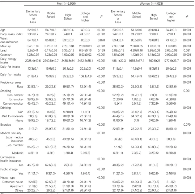
Table 3 demonstrates the characteristics of subjects according to level of education in both genders. According to level of education in both genders, there was similar to the trend of household income.
Men (n=3,966) Women (n=4,033)
Lowest Medium-
lowest Medium-
highest Highest P* Lowest Medium-
lowest Medium-
highest Highest P*
Age 54.1±1 43.7±0.5 40.8±0.4 42.3±0.4 <0.001 57.8±0.9 45.8±0.6 41.8±0.5 41.6±0.5 <0.001
Body mass index 23.5±0.2 24±0.1 24±0.1 24.5±0.1 <0.001 24.2±0.2 23.6±0.1 23±0.1 22.5±0.1 <0.001 Waist
circumference 83.7±0.5 84.1±0.4 83.9±0.3 85.2±0.3 0.007 81.8±0.5 79±0.4 77±0.3 75.4±0.3 <0.001
Mercury 5.38±0.2 5.26±0.13 5.91±0.24 6.84±0.19 <0.001 3.68±0.13 3.7±0.09 3.99±0.11 4.21±0.09 <0.001 Lead 3.15±0.07 2.94±0.05 2.74±0.05 2.73±0.04 <0.001 2.26±0.05 2.07±0.03 2.02±0.03 2.01±0.06 0.003 Cadmium 1.28±0.04 1.07±0.02 1.02±0.02 0.98±0.02 <0.001 1.45±0.04 1.23±0.02 1.16±0.02 1.16±0.02 <0.001 Daily energy intake 2107.6±56.4 2343.2±42.1 2429.8±37.2 2460.4±36.6 <0.001 1459.7±29.3 1642.4±23.9 1715.1±24.4 1728.5±23.6 <0.001 Daily fat intake 14.8±0.4 18.2±0.4 20±0.3 20±0.3 <0.001 13.8±0.5 16.5±0.3 17.7±0.3 18.5±0.3 <0.001 Daily fish intake 63.8±5 81±4.5 96.3±5.3 98.7±4.6 <0.001 36.2±2.5 48.2±3 55.8±2.8 60±2.7 <0.001
Residence areas <0.001 <0.001
Rural 27.6(2.9) 21(2) 19.8(1.8) 16.9(1.8) 0.009 28.2(2.7) 20.2(2) 16.5(1.7) 17.5(1.9)
Smoking 0.089
Non-smoker 20.7(2.1) 20.4(1.5) 24.1(1.5) 26.7(1.4) 88.7(1.6) 89.1(1) 91.6(1) 92.8(0.9) Ex-smoker 29.2(2.3) 28.8(1.7) 29.3(1.5) 31.6(1.5) 3.6(0.9) 4.5(0.7) 3.6(0.8) 3.2(0.6) Current-smoker 50.1(2.6) 50.8(1.8) 46.7(1.8) 41.8(1.7) 7.6(1.4) 6.5(0.8) 4.8(0.7) 4.1(0.7)
Drinking <0.001 <0.001
Non 24.4(2.3) 15.1(1.4) 11.7(1.1) 10.2(1) 49.4(2.7) 36.5(1.9) 28.8(1.7) 27.8(1.6) Mild to moderate 58.8(2.6) 63.9(1.9) 71.7(1.5) 70.5(1.5) 47.7(2.7) 62(1.8) 67.9(1.8) 71.4(1.6)
Heavy 16.8(1.9) 21(1.6) 16.6(1.3) 19.2(1.4) 2.9(0.8) 1.5(0.4) 3.3(0.7) 0.9(0.3)
Exercise <0.001 0.857
Yes 19.9(2.1) 27.9(1.7) 26.4(1.5) 31.4(1.6) 21.3(2.1) 21.2(1.5) 22.5(1.5) 22.9(1.6)
Medical security <0.001 <0.001
Local medical
insurance 41.2(2.6) 44.9(1.8) 37.5(1.8) 32.4(1.7) 41.9(2.5) 41.7(1.8) 40(1.8) 29.2(1.8) Job member
48.8(2.6) 52.8(1.8) 62.3(1.8) 67.5(1.7) 45.2(2.5) 56.2(1.8) 59.7(1.8) 70.3(1.8)
Medicaid 10(1.5) 2.2(0.5) 0.2(0.2) 0.1(0.1) 12.8(1.6) 2.2(0.5) 0.3(0.1) 0.5(0.3)
Commercial health
insurance <0.001 <0.001
Yes 37.9(2.6) 70.3(1.7) 84.1(1.3) 83.3(1.5) 44.8(2.6) 72.9(1.8) 81.7(1.4) 88.3(1.3)
Public charge <0.001 <0.001
Yes 15.1(1.8) 5.9(0.9) 2.1(0.6) 1.5(0.5) 17.5(1.7) 5.6(0.8) 3.1(0.7) 2.2(0.6)
House type <0.001 <0.001
Detached house 56.2(2.9) 45.8(2.2) 35(1.9) 31.7(2) 58.3(2.7) 39.4(2.1) 36.9(2.1) 31.1(2.1) Apartment 19.3(1.9) 24.4(1.4) 38.6(1.6) 49.7(1.9) 16.9(1.8) 30.4(1.8) 37.3(1.6) 51.3(2)
Others 24.5(2.6) 29.8(2.1) 26.4(1.9) 18.7(1.6) 24.8(2.3) 30.2(2.1) 25.9(1.9) 17.6(1.7) All values are mean±s.e. or percentage (s.e.).
*Calculated by Student’s t-test or Chi-square test.
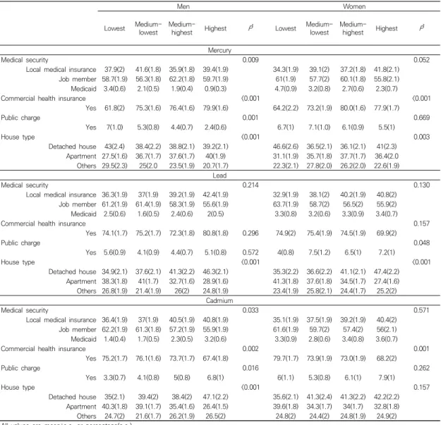
Table 2. Characteristics of study participants according to categories of household income Table 4 shows the relationship between income
level and blood heavy metal concentration according to the demographic characteristics.
Higher income people who lived in apartments indicated higher blood mercury concentration. In case of lead and cadmium more people of the high-income class who had higher blood lead and cadmium concentration lived in Detached house. All three metals showed relevance between income level and commercial health insurance. As the income level increased, the number of commercial health insurance
subscribers also increased.
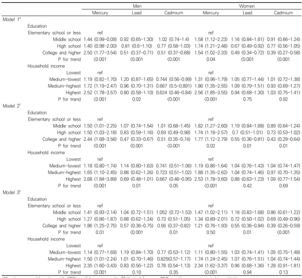
Table 5 depicts the ORs for the Heavy metals concentrations across the 4 categories of level of education and household income, using an elementary school or less level of education and the lowest household income as a reference, after controlling the effects of confounding factors on heavy metals concentrations.
According to level of education, Among men, the adjusted OR of mercury was 1.86-fold higher in the college and higher than in the reference in model 3. and the adjusted ORs of lead and
Men (n=3,966) Women (n=4,033)
Elementary School
or Less
Middle
School High
School
College higherand P*
Elementary School
Lessor
Middle
School High
School
College higherand P*
Age 62.5±0.6 54.7±0.8 38.8±0.4 40±0.3 <0.001 63.9±0.5 51.6±0.6 39.6±0.4 34.4±0.3 <0.001
Body mass index 23.5±0.2 24.1±0.2 24±0.1 24.5±0.1 <0.001 24.6±0.1 24.2±0.2 23±0.1 22±0.1 <0.001 Waist
circumference 84.7±0.4 85.8±0.5 83.5±0.3 85±0.3 0.870 83.4±0.4 80.5±0.5 76.6±0.3 73.7±0.3 <0.001 Mercury 3.46±0.08 3.25±0.07 2.78±0.04 2.59±0.03 <0.001 2.38±0.04 2.36±0.05 1.97±0.03 1.8±0.06 <0.001
Lead 5.9±0.41 6.17±0.26 5.35±0.12 6.54±0.16 0.139 3.89±0.13 4.39±0.16 3.98±0.08 3.65±0.09 0.081
Cadmium 1.38±0.04 1.23±0.03 1.02±0.02 0.93±0.02 <0.001 1.54±0.03 1.43±0.04 1.18±0.02 0.92±0.02 <0.001 Daily energy
intake 2028.4±49.6 2249.5±49.7 2438.8±34 2452.6±35.1 <0.001 1486.1±22.3 1665.6±37.4 1660.5±21 1777.6±23.7 <0.001 Daily fat intake 13.3±0.4 15.6±0.5 20.1±0.3 20.3±0.3 <0.001 11.9±0.4 14.5±0.4 18.3±0.3 20.6±0.3 <0.001 Daily fish intake 61.8±4.7 75.9±5.8 85.2±3.6 106.1±4.9 <0.001 35.3±2.3 51.4±4.9 56.6±2.2 59.4±2.9 <0.001
Residence areas <0.001 <0.001
Rural 33.8(3.1) 29.2(2.8) 19.5(1.7) 12.9(1.4) 28.9(2.3) 25.6(3.1) 16.8(1.6) 12.8(1.6)
Smoking <0.001 0.001
Non-smoker 14.7(1.9) 16.2(2) 25.1(1.2) 26.9(1.4) 92.2(1.2) 91.7(1.5) 88(1) 91.9(0.9)
Ex-smoker 39.9(2.6) 38.6(2.6) 25.7(1.3) 28.3(1.4) 2.5(0.6) 1.8(0.8) 4.6(0.6) 4.5(0.8) Current-smoker 45.4(2.7) 45.2(2.7) 49.1(1.4) 44.8(1.5) 5.3(1) 6.5(1.3) 7.3(0.9) 3.6(0.6)
Drinking <0.001 <0.001
Non 30.1(2.5) 16.5(2) 9.6(0.8) 11.1(1) 54.8(2.2) 32.4(2.7) 26.5(1.4) 25.4(1.6)
Mild to moderate 50(2.6) 63.8(2.6) 70.8(1.3) 72.5(1.5) 44.4(2.1) 64.6(2.7) 69.9(1.5) 73.4(1.6)
Heavy 19.9(2.2) 19.7(2.2) 19.6(1.2) 16.4(1.2) 0.7(0.3) 3(1) 3.6(0.6) 1.2(0.4)
Exercise <0.001 0.079
Yes 21(2.2) 25.9(2.6) 31.8(1.4) 24.5(1.4) 22.5(1.9) 23.2(2.3) 23.3(1.2) 18.5(1.4)
Medical security <0.001 <0.001
Local medical
insurance 40(2.7) 45(2.8) 43.2(1.5) 30.5(1.5) 36.2(2) 46.4(3.1) 43(1.6) 30(1.6)
Job member
55.2(2.7) 50.7(2.9) 55.2(1.5) 68.7(1.5) 57.5(2) 51.3(3.1) 53.8(1.7) 69.2(1.6)
Medicaid 4.8(1.1) 4.3(1) 1.5(0.4) 0.9(0.3) 6.3(1.1) 2.3(0.7) 3.2(0.5) 0.8(0.3)
Commercial
health insurance <0.001 <0.001
Yes 45.7(2.8) 62.6(2.8) 75(1.3) 84.3(1.2) 48.3(2.2) 77.7(2.4) 81(1.3) 88.2(1.1)
Public charge <0.001 <0.001
Yes 11.1(1.7) 6.3(1.3) 4.5(0.7) 1.8(0.4) 11.2(1.3) 6.8(1.4) 5.6(0.8) 2.4(0.5)
House type <0.001 <0.001
Detached house 52.6(3) 52.5(2.9) 40.7(1.8) 29.7(1.7) 53.6(2.2) 45.9(3.2) 34.7(1.8) 31.2(2) Apartment 21.3(2) 21.5(2.1) 31.9(1.3) 49.5(1.6) 23.7(1.6) 27(2.3) 38.7(1.4) 45.3(1.7)
Others 26.2(2.7) 26(2.8) 27.5(1.8) 20.8(1.6) 22.7(1.9) 27.1(2.9) 26.6(1.7) 23.5(1.8)
All values are mean±s.e. or percentage(s.e.).
*Calculated by Student’s t-test or Chi-square test.
Table 3. Characteristics of study participants according to categories of education level cadmium were 0.57 and 0.56-fold lower in the
college and higher than in the reference in model 3 separately. Among women, the adjusted OR of Mercury was 1.47-fold higher in those whose level of education was middle school in model 3. However, no significant association was found between education level and Mercury concentration. The adjusted ORs of lead and cadmium were 0.55 and 0.39-fold lower in the college and higher than in the reference in
model 3 separately. Concerning the level of lead and cadmium, are negatively associated higher exposures for lower education level in both genders. According to level of household income, Among men, the adjusted OR of Mercury in model 3 was 1.50-fold greater in those whose level of household income was medium-highest and 2.35-fold greater in those whose level of household income was highest. Among women, the adjusted OR of Mercury in model 3 was
Men Women
Lowest Medium-
lowest Medium-
highest Highest P* Lowest Medium- lowest Medium-
highest Highest P* Mercury
Medical security 0.009 0.052
Local medical insurance 37.9(2) 41.6(1.8) 35.9(1.8) 39.4(1.9) 34.3(1.9) 39.1(2) 37.2(1.8) 41.8(2.1) Job member 58.7(1.9) 56.3(1.8) 62.2(1.8) 59.7(1.9) 61(1.9) 57.7(2) 60.1(1.8) 55.8(2.1) Medicaid 3.4(0.6) 2.1(0.5) 1.9(0.4) 0.9(0.3) 4.7(0.9) 3.2(0.8) 2.7(0.6) 2.3(0.7)
Commercial health insurance <0.001 <0.001
Yes 61.8(2) 75.3(1.6) 76.4(1.6) 79.9(1.6) 64.2(2.2) 73.2(1.9) 80.0(1.6) 77.9(1.7)
Public charge 0.001 0.669
Yes 7(1.0) 5.3(0.8) 4.4(0.7) 2.4(0.6) 6.7(1) 7.1(1.0) 6.1(0.9) 5.5(1)
House type <0.001 0.003
Detached house 43(2.4) 38.4(2.2) 38.8(2.1) 39.2(2.1) 46.6(2.6) 36.5(2.1) 36.1(2.1) 41(2.3) Apartment 27.5(1.6) 36.7(1.7) 37.6(1.7) 40(1.9) 31.1(1.9) 35.7(1.8) 37.7(1.7) 36.4(2.0
Others 29.5(2.3) 25(2.0 23.5(1.9) 20.7(1.7) 22.3(2.1) 27.8(2.0) 26.2(2.0) 22.6(1.9)
Medical security Lead 0.214 0.130
Local medical insurance 36.3(1.9) 37(1.9) 39.2(1.9) 42.4(1.9) 32.9(1.9) 38.1(2) 40.2(1.9) 40.8(2) Job member 61.2(1.9) 61.4(1.9) 58.3(1.9) 55.6(1.9) 63.7(1.9) 58.7(2) 56.5(2) 55.9(2) Medicaid 2.5(0.6) 1.6(0.5) 2.4(0.6) 2(0.5) 3.3(0.8) 3.2(0.6) 3.3(0.9) 3.4(0.7)
Commercial health insurance 0.157
Yes 74.1(1.7) 75.2(1.7) 72.3(1.8) 80.8(1.8) 0.296 74.9(2) 75.4(1.9) 74.5(1.9) 69.9(2)
Public charge 0.048
Yes 5.6(0.9) 4.1(0.9) 4.4(0.7) 5.1(0.8) 0.572 4(0.8) 7.5(1.2) 6.5(1) 7.2(1)
House type <0.001 <0.001
Detached house 34.9(2.1) 37.6(2.1) 41.3(2.2) 46.3(2.1) 35.3(2.2) 36.6(2.2) 41.1(2.1) 47.4(2.2) Apartment 38.3(1.8) 41(1.7) 32.7(1.6) 28.9(1.6) 41.3(1.8) 37.6(1.8) 34.5(1.7) 27.4(1.6) Others 26.8(1.9) 21.4(1.9) 26(2) 24.8(1.9) 23.4(1.9) 25.8(2.1) 24.4(1.7) 25.2(2)
Cadmium
Medical security 0.033 0.571
Local medical insurance 36.4(1.9) 37(1.9) 40.5(1.9) 40.8(1.9) 35.1(1.9) 37.5(1.9) 39.2(1.9) 40.4(2) Job member 62.2(1.9) 61.3(1.8) 57.2(1.9) 55.9(1.9) 61.6(1.9) 59.7(2) 57.4(2) 56(2.1) Medicaid 1.4(0.4) 1.7(0.5) 2.3(0.5) 3.2(0.6) 3.3(0.9) 2.8(0.6) 3.4(0.8) 3.6(0.7)
Commercial health insurance 0.002 0.001
Yes 75.2(1.7) 76.1(1.6) 73.7(1.7) 67.4(1.8) 79.7(1.7) 73.9(1.9) 73.0(1.9) 68.2(2)
Public charge 0.016 0.262
Yes 3.3(0.7) 4.1(0.8) 5(0.8) 6.8(1) 6(1.1) 5.3(0.8) 6.1(1) 7.9(1)
House type <0.001 0.157
Detached house 35(2.1) 39.4(2) 38.4(2) 47.1(2.2) 35.6(2.1) 41.3(2.4) 41.3(2.2) 42.2(2.2) Apartment 40.3(1.8) 39.1(1.7) 35.4(1.6) 26.4(1.5) 39.6(1.8) 34.3(1.7) 34(1.7) 32.8(1.8)
Others 24.7(2) 21.6(1.7) 26.2(1.9) 26.5(2) 24.8(2) 24.4(2) 24.8(1.9) 24.9(2) All values are mean±s.e. or percentage(s.e.).
*Calculated by Student’s t-test or Chi-square test.
Table 4. The relationship between household income level and heavy metals concentration according to the demographic factors
1.74-fold greater in those whose level of household income was medium-highest and 2.34-fold greater in those whose level of household income was highest. However, no significant association was found between income level and lead and cadmium concentrations. Concerning the level of lead and cadmium, are negatively associated higher exposures for lower income level in both genders. We also analyzed the effects of other confounding factors on the level of heavy metals.
The blood mercury, lead, and cadmium concentration increased with age (people ≥20 aged) in both genders. Current smokers had a higher mercury level than non-smokers(OR, 1.34;
95% C.I., 1.022–1.759) and heavy drinkers had a higher mercury level than non-drinkers in both gender (OR, 2.39; 95% C.I., 1.630-3.496 in men;
OR, 3.71; 95% C.I., 1.705–8.073 in women). Weak associations with the dietary habits (fish consumption) were also observed. The adjusted
Men Women
Mercury Lead Cadmium Mercury Lead Cadmium
Model 1a
Education
Elementary school or less ref ref
Middle school 1.44 (0.99-0.09) 0.92 (0.65-1.30) 1.02 (0.74-1.4) 1.58 (1.12-2.23) 1.16 (0.84-1.61) 0.91 (0.66-1.24) High school 1.40 (0.98-2.00) 0.81 (0.6-1.10) 0.77 (0.58-1.03) 1.74 (1.21-2.48) 0.67 (0.49-0.92) 0.77 (0.56-1.05) College and higher 2.50 (1.77-3.54) 0.51 (0.37-0.71) 0.51 (0.37-0.68) 1.54 (1.02-2.33) 0.49 (0.34-0.72) 0.39 (0.27-0.58)
P for trend <0.001 <0.001 <0.001 0.04 <0.001 <0.001
Household income
Lowest ref ref
Medium-lowest 1.19 (0.82-1.70) 1.20 (0.87-1.65) 0.744 (0.56-0.99) 1.31 (0.96-1.79) 1.05 (0.77-1.44) 1.01 (0.72-1.38) Medium-highest 1.72 (1.19-2.47) 0.96 (0.70-1.31) 0.667 (0.5-0.891) 1.86 (1.35-2.55) 1.09 (0.79-1.51) 0.93 (0.69-1.27) Highest 2.52 (1.78-3.57) 0.80 (0.58-1.10) 0.624 (0.46-0.84) 2.56 (1.85-3.55) 0.94 (0.68-1.30) 1.03 (0.75-1.41)
P for trend <0.001 0.02 <0.001 <0.001 0.75 0.92
Model 2c
Education
Elementary school or less ref ref
Middle school 1.50 (1.01-2.25) 1.07 (0.74-1.54) 1.01 (0.68-1.45) 1.82 (1.27-2.60) 1.19 (0.84-1.68) 0.89 (0.64-1.24) High school 1.50 (1.03-2.18) 0.83 (0.59-1.16) 0.69 (0.49-0.98) 1.74 (1.18-2.57) 0.7 (0.51-1.01) 0.73 (0.53-1.02) College and higher 2.44 (1.68-3.56) 0.47 (0.33-0.67) 0.51 (0.35-0.74) 1.77 (1.12-2.79) 0.55 (0.36-0.81) 0.43 (0.29-0.64)
P for trend <0.001 <0.001 <0.001 0.02 0.01 0.01
Household income
Lowest ref ref
Medium-lowest 1.18 (0.80-1.74) 1.14 (0.80-1.63) 0.741 (0.51-1.06) 1.19 (0.86-1.64) 1.04 (0.76-1.43) 1.04 (0.74-1.47) Medium-highest 1.65 (1.10-2.45) 0.88 (0.62-1.26) 0.723 (0.51-1.02) 1.88 (1.35-2.62) 1.04 (0.74-1.46) 0.97 (0.70-1.35) Highest 2.68 (1.84-3.89) 0.69 (0.48-1.01) 0.667 (0.46-0.95) 2.53 (1.78-3.60) 0.88 (0.63-1.23) 1.09 (0.77-1.54)
P for trend <0.001 0.01 0.05 <0.001 0.42 0.69
Model 3c
Education
Elementary school or less ref ref
Middle school 1.41 (0.93-2.14) 1.04 (0.72-1.51) 1.052 (0.72-1.53) 1.47 (1.02-2.11) 1.18 (0.83-1.68) 0.86 (0.61-1.22) High school 1.27 (0.86-1.87) 0.88 (0.62-1.24) 0.73 (0.51-1.05) 1.34 (0.89-2.01) 0.72 (0.50-1.02) 0.69 (0.49-0.96) College and higher 1.86 (1.25-2.75) 0.57 (0.36-0.75) 0.56 (0.37-0.82) 1.21 (0.76-1.93) 0.55 (0.36-0.84) 0.39 (0.26-0.59)
P for trend 0.01 <0.001 0.01 0.50 0.01 <0.001
Household income
Lowest ref ref
Medium-lowest 1.14 (0.77-1.69) 1.19 (0.84-1.70) 0.77 (0.53-1.12) 1.11 (0.80-1.55) 1.03 (0.74-1.41) 1.05 (0.75-1.48) Medium-highest 1.50 (1.01-2.24) 1.01 (0.70-1.46) 0.825(0.57-1.17) 1.74 (1.24-2.45) 1.07 (0.76-1.51) 1.04 (0.74-1.44) Highest 2.35 (1.60-3.43) 0.83 (0.56-1.22) 0.78 (0.54-1.13) 2.34 (1.62-3.37) 0.96 (0.68-1.36) 1.28 (0.91-1.81)
P for trend <0.001 0.10 0.35 <0.001 0.94 0.13
All values are odds ratios with 95% confidence intervals. aAdjusted for age, BMI, residence areas, smoking, drinking, exercise.
bAdditionally adjusted for daily fish intake
cAdditionally adjusted education for household income, household income for education ref(reference)
Table 5. Odds ratios and 95% confidence intervals of the level of Heavy metals among Korean adults across categories of SES
OR of fish consumption was 1.001; 95% C.I., 1.001-1.002 in men and the adjusted OR of fish consumption was 1.003; 95% C.I., 1.001-1.004 in women. Finally, Current smokers had a higher lead and cadmium level than non-smokers in both genders and mild to moderate drinkers had a higher lead level than non-drinkers (OR, 1.96;
95% C.I., 1.374-2.805) in men; OR, 1.305; 95%
C.I., 1.027–1.659 in women).
This study showed that education and income as indicators of SES were associated with lead,
cadmium, and mercury concentration in blood.
The blood levels of lead and cadmium were higher when educational levels were lower and the blood concentrations of mercury increased as levels of education were higher in men. It showed that women have a similar trend with men but there was no statistical significance in the case of mercury.
The blood levels of mercury were higher when incomes levels were higher and the blood concentrations of lead and cadmium showed the
opposite tendency as compared with mercury in men. It showed that women have a similar trend with men but there was statistical significance in the case of mercury. This result agrees with other studies that have also reported the same results.
Low SES was found to be related to high lead and cadmium blood concentrations while higher blood concentrations of mercury was found when the SES is high[21,25,26,29,30]. It is also reported that this tendency of blood level Mercury being high when the SES is high is associated with the consumption of fish [12,13,21,22,31,33]. This agrees with the results from this study, that higher income level and education level is related to higher consumption of fish showing higher mercury concentration in blood. Furthemore, Few studies have examined association between Lead and Cadmium poisoning and the poor lifestyle such as smoking and drinking at low SES [16-20,34]. This study found the Current smokers had a higher lead and cadmium level than non-smokers in both genders. The previous studies showed that the number of smoker and smoking at home were positively correlated with lead and cadmium concentrations in hair[20,34]. This study showed that as income level increased, blood mercury level was higher among people who lived in the apartments and blood lead and cadmium levels were higher among people who lived in the Detached house and this was consistent with the studies that reported SES such as maternal smoking, outdoor activity level of the mother, and quality of their apartments are related to blood lead concentrations[29]. Also in this study, blood cadmium level was higher when the education level was lower. Some studies point out that the blood cadmium level was correlated with maternal education level and teenage children with college graduates have higher levels of cadmium in their blood than those with elementary school graduates[35]. Other study showed that higher maternal education level is
associated with consumption of vegetables and that a mother with higher education level consumed more vegetables[35]. In this study however, did not consider relationship between maternal education level and the maternal vegetable dietary so further studies related to maternal education level and maternal vegetable dietary is required.
In this study, it was significant that even if cross-sectional study to infer a cause-and-effect relationship is difficult, it was an opportunity to highlight the importance of socioeconomic health disparities by examining the relevance for the socioeconomic status and blood concentrations of heavy metals, using the Korean National Health and Nutritional Examination Survey.
In conclusion, this study showed that education and income as indicators of socioeconomic status were inversely associated with lead and cadmium concentration, and were linked with higher lead levels in Korean adult population. At the point of an increase in the prevalence of heavy metal concentrations in the blood, it is believed that a national public health policy will be needed to address the inequity of health due to socioeconomic factors.
REFERENCES
[1] F. Fuentes-Gandara, J. Pinedo-Hernndez, J.
Marrugo-Negrete & S. Dez. (2018). Human health impacts of exposure to metals through extreme consumption of fish from the Colombian Caribbean Sea. Environmental geochemistry and health, 40(1), 229-242.
[2] R. Figueroa, D. Caicedo, G. Echeverry, M. Pea & F.
Mndez. (2017). Socioeconomic status, eating patterns, and heavy metals exposure in women of childbearing age in Cali, Colombia, Biomedica: revista del Instituto Nacional de Salud, 37(3), 341-352.
[3] S. M. Park & B. K. Lee. (2013). Body fat percentage and hemoglobin levels are related to blood lead, cadmium, and mercury concentrations in a Korean Adult Population (KNHANES 2008-2010). Biological trace element research, 151(3), 315-323.
[4] I. Y. Yoo. (2014). The Blood levels of lead, mercury, and cadmium and metabolic syndrome of Korean adults. Journal of The Korean Society of Living Environmental System, 21(2), 251-259.
[5] X. Xufeng, Z. Lou, G. Christakos, Z. Ren, Q. Liu & X.
Lv. (2018). The association between heavy metal soil pollution and stomach cancer: A case study in Hangzhou city, China. Environmental geochemistry and health, 40(6), 2481-2490.
[6] R. Chowdhury et al. (2018). Environmental toxic metal contaminants and risk of cardiovascular disease:
systematic review and meta-analysis. bmj, 362, k3310.
[7] A. Jan, M. Azam, K. Siddiqui, A. Ali, I. Choi & Q. Haq.
(2015). Heavy metals and human health: mechanistic insight into toxicity and counter defense system of antioxidants. International journal of molecular sciences, 16(12), 29592-29630.
[8] K. Jomova & M. Valko. (2011). Advances in metal-induced oxidative stress and human disease.
Toxicology, 283(2-3), 65-87.
[9] A. Bhatnagar. (2006). Environmental cardiology:
studying mechanistic links between pollution and heart disease. Circulation research, 99(7), 692-705.
[10] P. Muntner, A. Menke, K. B. DeSalvo, F. A. Rabito & V.
Batuman. (2005). Continued decline in blood lead levels among adults in the United States: the National Health and Nutrition Examination Surveys. Archives of Internal Medicine,165(18), 2155-2161.
[11] J. W. Seo et al. (2015). Trend of blood lead, mercury, and cadmium levels in Korean population: data analysis of the Korea National Health and Nutrition Examination Survey. Environmental monitoring and assessment, 187(3), 1-13.
[12] W. McKelvey et al. (2007). A biomonitoring study of lead, cadmium, and mercury in the blood of New York city adults. Environmental Health Perspectives, 115(10), 1435-1441.
[13] C. M. L. Carvalho, A. I. N. M. Matos, M. L. Mateus, A.
P. M. Santos & M. C. C. Batoréu. (2008). High-fish consumption and risk prevention: assessment of exposure to methylmercury in Portugal. Journal of Toxicology and Environmental Health, Part A, 71(18), 1279-1288.
[14] N. S. Kim & B. K. Lee. (2011). National estimates of blood lead, cadmium, and mercury levels in the Korean general adult population. International archives of occupational and environmental health, 84(1), 53-63.
[15] K. Nomiyama, H. Nomiyama, S. J. Liu, Y. X. Tao, T.
Nomiyama & K. Omae. (2002). Lead induced increase of blood pressure in female lead workers.
Occupational and Environmental Medicine, 59(11), 734-738.
[16] J. S. Oh & S. H. Lee. (2015). Pb, Hg and Cd concentration of blood and exposure-related factors.
Korea Academy Industrial Cooperation Society, 16(3), 2089-2099.
[17] H. Bjermo et al. (2013). Lead, mercury, and cadmium in blood and their relation to diet among Swedish adults. Food and Chemical Toxicology, 57, 161-169.
DOI: http://dx.doi.org/10.1016/j.fct.2013.03.024 [18] B. R. Lee & J. H. Ha. (2011). The Effects of Smoking
and Drinking on Blood Lead and Cadmium Levels:
Data from the Fourth Korea National Health and Nutrition Examination Survey. Korean J Occup Environ Med, 23(1), 31-41.
[19] J. Y. Shin, J. M. Kim & Y. R. Kim. (2012). The association of heavy metals in blood, fish consumption frequency, and risk of cardiovascular diseases among Korean adults: The Korea National Health and Nutrition Examination Survey(2008-2010).
Korean J Nutr, 45(4), 347-361.
DOI: http://dx.doi.org/10.4163/kjn.2012.45.4.347 [20] T. A. Ozden et al. (2007). Elevated hair levels of
cadmium and lead in school children exposed to smoking and in highways near schools. Clinical biochemistry, 40(1-2), 52-56
[21] M. Vrijheid et al. (2012). Socioeconomic status and exposure to multiple environmental pollutants during pregnancy: evidence for environmental inequity?. J Epidemiol Community Health, 66(2),106-113.
[22] B. Morrens et al. (2012). Social distribution of internal exposure to environmental pollution in Flemish adolescents. International journal of hygiene and environmental health, 215(4), 474-481.
[23] L. S. Morales, P. Gutierrez & J. J. Escarce. (2005).
Demographic and socioeconomic factors associated with blood lead levels among mexican-american children and adolescents in the united states. Public Health Reports, 120(4), 448-454.
[24] H. J. Jin & S. M. Cho. (2016). Estimation of Socio-economic Costs of Illness due to Blood Concentration of Heavy Metals in Koreans among the Public . Health and social welfare review, 36(4), 508-536.
[25] J. L. Peters et al. (2011). Childhood and adult socioeconomic position, cumulative lead levels, and pessimism in later life: the VA Normative Aging Study.
American journal of epidemiology, 174(12), 1345-1353.
[26] S. M. Bernard & M. A. McGeehin. (2003). Prevalence of blood lead levels≥5µg/dL among US children 1 to 5 years of age and socioeconomic and demographic factors associated with blood of lead levels 5 to 10µg/dL, Third National Health and Nutrition Examination Survey, 1988-1994. Pediatrics, 112(6), 1308-1313.
[27] J. Kim, M. Shin, S. Kim, J. Seo, H. Ma & Y. J. Yang.
(2017). Association of iron status and food intake with blood heavy metal concentrations in Korean
adolescent girls and women : Based on the 2010~2011 Korea National Health and Nutrition Examination Survey. Journal of Nutrition and Health, 50(4), 350-360.
[28] M. H. Kang, S. M. Park, D. N. Oh, M. H. Kim & M. K.
Choi. (2013). Dietary nutrient and food intake and their relations with serum heavy metals in osteopenic and osteoporotic patients. Clin Nutr Res, 2(1), 26-33.
[29] K. Osman, J. E. Zejda, A. Schutz, D. Mielzynska, C. G.
Elinder & M. Vahter. (1998). Exposure to lead and other metals in children from Katowice district, Poland, International archives of occupational and environmental health, 71(3), 180-186.
[30] S. Elreedy, N. Krieger, P. B. Ryan, D. Sparrow, S. T.
Weiss & H. Hu. (1999). Relations between individual and neighborhood-based measures of socioeconomic position and bone lead concentrations among community-exposed men: the Normative Aging Study.
American Journal of Epidemiology, 150(2), 129-141.
[31] J. M. Hightower & D. Moore. (2003). Mercury levels in high-end consumers of fish. Environmental health perspectives, 111(4), 604-608.
[32] E. Oken et al. (2008). Maternal fish intake during pregnancy, blood mercury levels, and child cognition at age 3 years in a US cohort. American journal of epidemiology, 167(10), 1171-1181.
[33] S. Lim, H. U. Chung, D. Paek. (2010). Low dose mercury and heart rate variability among community residents nearby to an industrial complex in Korea.
Neurotoxicology, 31(1), 10-16.
[34] M. A. Serdar et al. (2012). The correlation between smoking status of family members and concentrations of toxic trace elements in the hair of children.
Biological trace element research, 148(1), 11-17.
[35] E. Barany et al. (2002). Trace elements in blood and serum of Swedish adolescents: relation to gender, age, residential area, and socioeconomic status.
Environmental research, 89(1), 72-84.
김 정 현(Junghyun Kim) [정회원]
· 2009년 8월 : 서울대학교 보건학과 (보건학석사)
· 2012년 2월 : 서울대학교 보건학과 (보건학박사수료)
· 관심분야 : 지역사회보건
· E-Mail : [email protected]
조 영 태(Youngtae Cho) [정회원]
· 1999년 5월 : University of Texas-Austin(사회학 석사)
· 2002년 8월 : University of Texas –Austin(인구학 박사)
· 2002년 9월 ∼ 2004년 7월 : Utah State University 사회학과 조교수
· 2004년 8월 ∼ 현재 : 서울대학교 보건대학원 교수
· 관심분야 : 인구와 미래사회, mHealth, 인구와 개발, 비 즈니스 인구학
· E-Mail : [email protected]