Simulation Model of Dual-Species Biofilm Growth in Hydrodynamic Flow

유체 흐름 안에서 두 종의 생물막 성장 시뮬레이션 모델

전원주¹･ 이상희^1†

Simulation Model of Dual-Species Biofilm Growth in Hydrodynamic Flow

Wonju Jeon ･ Sang-Hee Lee

ABSTRACT

In rivers and streams, biofilms are thin layers of greenish-brown slime attached to rocks, plants, and other surfaces.

Biofilms play key roles in primary production and cycling of nutrients, water quality remediation, suspended sediment removal, and energy flow to higher trophic levels. In the present study, we developed a two-dimensional cellular automata model to simulate mixed biofilms of toxin-sensitive and toxin-producing species in hydrodynamic flow. The flow was generated by a stochastic process for uniform flow and by using the Navier-Stokes equation for non-uniform flow. Minimized local rules governing reproduction and mortality of the species were executed in the self-organizing processes to elucidate interactions between toxin-producing and toxin-sensitive species in competition over nutrients.

We briefly discuss the morphology of the simulated biofilm under different flow conditions.

Key words : Biofilm; species competition; bacterial interaction; cellular automata model

요 약

하천에서, 생물막은 녹갈색의 얇은 막의 형태로 돌, 식물, 그리고 기타 구조물의 표면에 부착되어 있다. 생물막은 주로 영양 물의 순환, 수질정화, 바닥 침전물 제거, 그리고 먹이사슬내의 에너지 흐름에 매우 중요한 역할을 한다. 본 연구에서, 우리는 유체 흐름 안에서, 독소-생산 종과 독소-민감 종의 복합적 생물막을 전산 모사하는 모델을 개발하였다. 유체 흐름으로는 균일한 흐름과 불 균일한 흐름 두 가지를 고려하였다. 균일한 흐름은 확률 프로세스로 구현되었으며, 불 균일한 흐름은 나비어-스톡스 방정식으로 구현되었다. 모델에서, 독소-생산종과 독소-민감종 간의 상호작용을 고려하기 위해, 종 개체의 번식률과 사망률이 고려되어졌다. 우리는 서로 다른 두 유체 흐름 내에서 전산 모사 되어진 생물막의 구조적 형상에 대해서 간략히 논의 하였다.

주요어 : 생물막, 종간경쟁, 박테리아 상호작용, 세포자동자 모델

*This study was carried out with the support of “Cooperative Research Program for Agricultural Science & Technology Development(project No. 20100401-030-079-001-00-00)”, RDA, Republic of Korea, and partly supported by National Institutes for Mathematical Sciences.

접수일(2010년 12월 18일), 심사일(1차 : 2011년 3월 14일), 게재 확정일(2011년 3월 21일)

1)국가수리과학연구소 융복합수리과학부

주 저 자: 전원주 교신저자: 이상희

E-mail; [email protected]

1. 서 론

Biofilms are assemblages of microorganisms in which cells adhere to each other and/or to a surface. They can

be readily established at any interface on living organisms

(e.g., teeth, dental plaque, plant leaves), non-living organisms

(e.g., soil, stones in riverbeds, marine and freshwater

sediments), and non-natural structures(e.g., filters, ship

hulls, pipelines, bioreactors)

. To synthesize biofilms

and integrate our knowledge about their behavior,

mathematical models have been developed over the past

three decades. Early models in the 1970s simulated

biofilms as homogeneous steady-state films of a single

species, mainly with regard to one-dimensional mass

transport and biochemical reactions

. These models

later evolved to multi-species substrates and multi-substrate

biofilm models

. Since the early 1990s, attention has

전원주 ･ 이상희

been drawn focused on the morphological development of highly irregular and heterogeneous spatial structures

. Recently, by increasing computational power, morphological development of biofilms in 2 and 3 dimensions has been extensively studied with self-generative algorithms

. These models are generally suitable for representing aggregate biofilm activity within hydrodynamic flows.

More recently, integrative models have been proposed to incorporate the whole spectrum of spatial and temporal dynamics of biofilm growth, encompassing transport processes, population growth, and detachment to various extents

. In the integrative models, biofilm structure has been regarded as an emergent property through a bottom-up approach because the formation of the complex community emerges as a result of the interactions of components in response to environmental changes.

Biofilm morphology is closely related to its functional interactions with the surrounding environment, and external mass transfer phenomena contribute to such interactions.

In addition, the resulting local and global morphological structures contribute to the dynamics of biofilm development.

This reflects the processes of a specimen’s growth and death. Thus, improved methods for characterization of biofilm structures are needed

. However, only few advances have been achieved. Zhang and Bishop

evaluated the internal porosity of biofilm voids, whereas fractal geometry has been employed for characterization of both pore space and biomass

.

In the present study, we constructed a cellular automata model to address interactions of 2 species under the constraints of allelopathy. Allelopathy has been experi- mentally tested in various species, including marine algal species both in vitro and in situ

. Among various organisms, allelopathy in bacteria has been extensively investigated. For example, bacteria produce toxic substances known as bacteriocins that kill or inhibit competing bacteria of different genotypes, whereas bacteria that are capable of producing toxins are immune to their own action. Allelopathy is in fact prevalent in nature and may even be considered as playing a “necessary”

role in the chemical communication networks between plants and other organisms

.

In this study, we did not compare the simulation

results with experimental data to test if the model we proposed in this study was valid. This is because we wish to avoid digression of the focus of this study. In the near future, we will undertake validation by performing comparisons with empirical data as well as with other mathematical models.

2. Model Description

2.1 Cellular automata

The cellular automata model is described in a two- dimensional system with an L×L site grid, where L(=200) is the system size. The update is carried out synchronously in the model with respect to specimens of bacteria, nutrients, and toxicants. Each bacterial specimen, nutrient, and toxicant can move to only 1 site per time- step. Each interior site(i, j) (where i = 2,…,n-1 and j

= 2,…,n-1) has 8 immediate neighbors(i-1, j-1), (i-1, j), (i-1, j+1), (i, j-1), (i, j+1), (i+1, j-1), (i+1, j) and (i+1, j+1). In order to decide the progression of growth of biofilm from the previous step, we have defined a set of rules described below..

2.2 Occupation of Sites

Each site can be occupied by any 1 of 4 possible subjects: a toxin-producing specimen, toxin-sensitive specimen, nutrient, or toxicant. In addition, a site may be occupied by 1 toxicant and 1 nutrient, or by 1 toxicant and 1 toxin-producing specimen. Thus, there are 6 different occupancies for a given site.

2.3 Bacterial growth

Cell-division occurs for the toxin-sensitive(or toxin- producing) specimens with a defined probability(in this case, p=1) when their neighboring sites are occupied by at least 1 nutrient(Fig. 1(a), (b)).

When more than 1 toxin-producing(and/or toxin- sensitive) specimen competes with others in the group for a nutrient, the occupant of the nutrient is determined randomly(i.e., coin toss) (Fig. 1 (c), (d), (e)).

2.4 Toxic effect

When 1 or more toxin-sensitive specimens are present

Fig. 1. All possible configurations when each species can encounter a toxicant or a nutrient. The arrow signs indicate the direction of growth of each species or the direction of movement of nutrients and toxicants. The large solid octagon, large octagon, small solid octagon, and small octagon represent toxin-producing species, toxin-sensitive species, toxicants, and nutrients, respectively

Fig. 2. Multiplication process of each species toward one of the unoccupied neighboring sites during 1 iteration time stept>t+1

in the immediate neighboring sites of toxin, death of the toxin-sensitive species by toxicants will occur due to diffusion of the toxicant(Fig. 1 (f), (g)).

When more than 1 toxicant is present in the neighboring sites of a toxin-sensitive specimen, the coin toss rule is applied to determine which toxicant kills the toxin- sensitive specimens(Fig. 1(h)).

The site of a toxin-producing specimen can be shared with a toxicant(Fig. 1 (i), (j)). In this case, there is no

interaction between the toxicant and the toxin-producing specimen.

When the toxin-producing specimen is present at one

of the neighboring sites of a site occupied by a nutrient,

the uptake of the nutrient is carried out by the progeny of

the toxin-producing specimen. A toxicant is immediately

produced by the progeny of the toxin-producing specimen

and occupies one of the neighboring sites of the toxin-

producing specimen(Fig. 2 (a)).

전원주 ･ 이상희

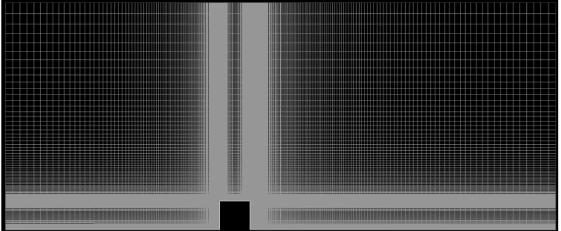
Fig. 3. Computational domain for the flow consisting of 3 blocks: bottom space, near the edge corner of obstacle, and upper space. The black rectangle-shaped box represents the simplified obstacle

When toxicants(and/or nutrients) are present at 1 or more sites of the neighboring toxin-sensitive specimen sites, cell division occurs before diffusion of toxicants or nutrients. Immediately after progenies are produced, the toxicant either diffuses to an empty site(or to the site occupied by toxin-producing specimen) or kills the toxin-sensitive specimen or its progeny(Fig. 2 (b)).

When a neighboring toxin-sensitive specimen site is simultaneously occupied by a nutrient and a toxicant, cell division occurs before diffusion of the toxicant(Fig. 2 (c)).

2.5 Hydrodynamic Flow

2.5.1 Uniform flow

To describe the uniform flow, we assigned a drift probability, P

, to each cell. In this study, the value of P

was set to 1/3.

2.5.2 Non-uniform flow

Two equations were used to simulate non-uniform flow: a continuity equation satisfying the mass conservation law and the Navier-Stokes equation in two-dimensions concerning the conservation of fluid momentum. The flow is generated in a space different from the grid space for bacterial species, nutrients, and toxicants. The space for the flow consists of 3 blocks, and the total number of 80,032 grids in a rectangular mesh is used.

A rectangle-shaped obstacle was introduced to simply

describe a small structure at the bottom of the stream.

The flow is strongly influenced by the obstacle. Thus, to capture the flow properties in detail around the obstacle, the grid points are clustered along the bottom surface, near the edge corner of the obstacle and the presumed vortex trajectory(see Fig. 3). The algorithm is implemented in the delta form with trapezoidal temporal differencing and central spatial differencing, which have second-order temporal and spatial accuracies. Fourth-order explicit and second-order implicit numerical damping is used to eliminate spurious numerical oscillations. The boundary conditions are imposed as follows. On the bottom surface and the obstacle surface, the no-slip condition is applied to the velocity. The inflow boundary condition is given by uniform velocity input, and the outflow boundary conditions are given by flux conditions. Fig. 4 shows that our simulation model successfully captures the flow flux around the obstacle.

2.6 Particle Movement

In uniform flow, particles, nutrients, and toxicants behave as drift random walks on the grid space due to the drift probability. On the other hand, in non-uniform flow, the particles move according to Newton’s equation of motion as follows:

) ( 6 ) 2 (

) 1

( i f i i i i

f i f p i

p V u a V u

dt m d dt m du g m dt m

m dV = − + − − − πμ −

Fig. 4. Flow dynamics for 200 simulation iterations. The arrow lines represent flow flux

Here, m

is the mass of a particle, m

is the mass of fluid displaced by the particle, g

is the gravitational acceleration, and a represents the radius of a particle.

The terms on the right side of the equation represent the force due to buoyancy, fluid acceleration, inertia of added mass, and Stokes drag by skin friction, respectively.

2.7. Initial Bacterial Distribution

Twenty toxin-sensitive and 10 toxin-producing specimens were initially generated at periodic positions on the bottom edge of the arrays(x-positions of toxin-sensitive specimens:

10, 20, 30,…, 200; x-positions of toxin-producing specimens:

5, 25, 45,…, 185). An initial “inoculum” of nutrients was introduced with a random distribution on the square lattice. The initial occupancy of the nutrient at each site is determined by thresholding, which is based on the probability C

:

⎩ ⎨

⎧ <

= otherwise

C j i rand j when

i

N

, 0

) , ( ,

) 1 , (

where N is the total number of nutrient particles, rand(i, j) means the randomly generated number at the site(i, j).

2.8 Flow-Chart of the Present Biofilm Model

Flow-Chart of the Biofilm Model

전원주 ･ 이상희

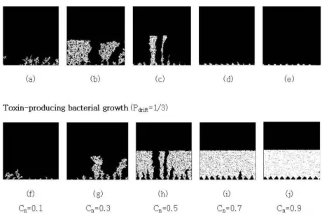
Fig. 5. Typical patterns of biofilm growth. The base was inoculated with a repeating sequence of 20 toxin-sensitive species and 10 toxin-producing species at Pdrift = 1/3. (a)-(e) Toxin-sensitive bacterial growth at nutrient concentrations Cn=0.1,0.3,0.5,0.7, and 0.9. (f)-(j) Toxin-producing bacterial growth at nutrient concentrations Cn=0.1,0.3.0.5,0.7,and0.9

The whole procedures of the biofilm model explained in section 2 is summarized by a flow-chart for reader’s convenience. The first and the second modules were explained in section 2.5 and 2.6, respectively. And, the third module was explained in section 2.1-4 and 2.7.

3. Simulation Results

The morphological structure of simulated biofilm in uniform flow at different nutrient concentrations(C

= 0.1, 0.3, 0.5, 0.7, and 0.9) is shown in Fig. 5. When nutrient concentrations are low with C

= 0.1 at P

= 1/3, the growth rate of population of both toxin-sensitive bacteria(Fig. 5 (a)) and toxin-producing bacteria(Fig. 5 (f)) was low. This is because the specimens could not readily use nutrients for growth. At higher levels of C

=0.7 and 0.9, the growth rate of population of the toxin-sensitive bacteria(Fig. 5 (d) and (e)) was low, but that of toxin-producing bacteria(Fig. 5 (i) and (j)) was high. As C

was increased from 0.1 to 0.5, vertical growth was more apparent both for toxin-sensitive(Fig. 5 (a), (b), and (c)) and toxin-producing bacteria(Fig. 5 (f), (g), and (h)), but the resulting patterns were not clearly

distinguishable between toxin-sensitive and toxin-producing bacteria. This is because the toxicants produced by the toxin-producing bacteria limited the growth of toxin- sensitive bacteria during growth. Some of the toxin- sensitive bacteria were killed during the growth phase.

When the nutrient concentration C

was increased from 0.5 to 0.9, the growth patterns were different between toxin- sensitive and toxin-producing bacteria. Toxin-producing species were prevalent(Fig. 5 (h), (i), and (j)), whereas toxin-sensitive species were excluded(Fig. 5 (c), (d), and (e)) from the space because they were killed by the toxin-producing species.

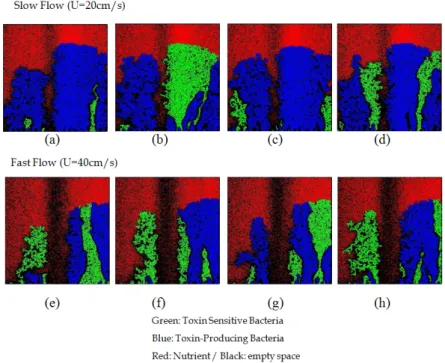
The morphological structure of simulated biofilm in non-uniform flow at C

= 0.1, 0.2, 0.3, and 0.4 is shown in Fig. 6. The obstacle was located centrally at the bottom. The upper area of the obstacle is empty(black).

This is because nutrient particles are rapidly consumed

in this area relative to other areas. The values of initial

flow speed were 20 cm/s(slow flow) and 40 cm/s(fast

flow). This strong vortex forms a circulation zone behind

the obstacle(see Fig. 4), and this circulation zone plays

a role in dispersing the nutrient particles far away from

the obstacle. Thus, biofilm growth, which strongly depends

Fig. 6. Typical patterns of biofilm growth. The base was inoculated with a repeating sequence of 20 toxin-sensitive species and 10 toxin-producing species in slow and fast flow. (a)-(d): Biofilm growth pattern in slow flow at Cn=0.1,0.2,0.3, and 0.4.(e)-(h) : Biofilm growth pattern in fast flow at Cn=0.1,0.2,0.3, and 0.4

on the presence of nutrients, was found to be significantly different in the areas in front of and behind the obstacle.

4. Conclusions

In this study, we developed a biofilm growth model with allelopathic effects on uniform and non-uniform flows. Our biofilm model is capable of simulating spatial and temporal growth dynamics under different flows.

Growth dynamics were distinguished between toxin- sensitive species and toxin-producing species. This model can be a useful tool for the analysis of biofilms under various flow conditions and may also be used as a tool for expressing the impact of internal stresses caused by environmental changes on structural changes in complex relationships among populations.

Appendix

A1. Equations of Hydrodynamic Simulation

To simulate the biofilm growth in water as realistic

as possible, it is essential to solve the equations of fluid mechanics. Two essential equations in fluid mechanics are continuity equation, Eq.(1), satisfying the mass conservation law and the Navier-Stokes equation, Eq.(2), governing the conservation of fluid momentum.



 _

 _  

(1)



 _  _

 __ _ _  

(2)

Here,

is the density,

is the velocity component,



is the hydrodynamic pressure,

is the Kronecker delta(

=1 for i=j, else

=0). And,

is the viscous shear stress defined as below.

_ 



 

_

 _

_



_

_





A2. Significance of Hydrodynamic Simulation

By numerically solving the Eq.(1) and Eq.(2) with

high resolution grid illustrated in Fig. 3, we calculate

전원주 ･ 이상희

the flow variables such as pressure and velocity in the flow field with high precision. In many biofilm models, the water flow was not considered in the biofilm process and the temporal variations of flow variables have been completely neglected. However, the accurate flow simulation is important not only in the formation of biofilm architecture but also in the trajectories of organic particles transported in the flow, which significantly influences the growth pattern of biofilm on the substratum.

REFERENCES

1. Costerton, J.W., Lewandowski, Z., Caldwell, D.E., Korber, D.R., and Lappin-Scott H.M., “Microbial biofilms,” Annual Review of Microbiology. vol. 49, pp. 711-745, 1995.

2. Stoodley, P., Yang, S., Lappin-Scott, H., and Lewandowski, Z., “Relationship between mass transfer coefficient and liquid flow velocity in heterogeneous biofilms using microelectrodes and confocal microscopy,” Biotechnology and Bioengineering. vol. 56, pp. 681-688, 1997.

3. Tolker-Nielsen, T. and Molin, S., “Spatial organization of microbial biofilm communities,” Microbial Ecology.

vol. 40, pp. 75-84, 2000.

4. Ames, W.F., Numerical methods for partial differential equation, 2nd ed, London: Thomas Nelson and Sons, 1977.

5. Shuler, M.L., Leung, S.K., and Dick, C.C., “A mathematical model for the growth of a single bacterial cell,” Annals of the New York Academy of Sciences. vol. 326, pp.

35-55, 1979.

6. Bryers, J.D. and Characklis, W.G., “Processes governing primary biofilm formation,” Biotechnol. Bioeng. 24, pp.

2451-2476, 1982.

7. Characklis, W.G., Biofilm development: a process analysis.

In Microbial Adhesion and Aggregation, (ed. K.C. Marshall), pp. 137-158, Springer, Berlin, 1984.

8. Gjaltema, A., Arts, P.A.M., van Loosdrecht, M.C.M., Kuenen, J.G., and Heijnen, J.J., “Heterogeneity of biofilms in rotating annular reactor: occurrence, structure, and consequences,” Biotechnology and Bioengineering, vol. 44, pp. 194-204, 1994.

9. Wimpenny, J.W.T. and Colasanti, R., “A unifying hypothesis for the structure of microbial biofilms based on cellular

automaton models,” FEMS Microbiology Ecology. vol.

22, pp. 1-16, 1997.

10. Hermanowicz and S. W., “A simple 2D biofilm model yields a variety of morphological features,” Mathematical Biosciences. vol. 169, pp. 1-14, 2001.

11. Noguera, D.R., Okabe and S., and Picioreanu, C., “Biofilm modeling: Present status and future directions,” Water Science and Technology. vol. 39, pp. 273-278, 1999.

12. Noguera, D.R., Pizarro, G., Stahl, D.A., and Rittmann, B.E., “Simulation of multispecies biofilm development in three dimensions,” Water Science and Technology.

vol. 39, pp. 123-130, 1999.

13. Eberl, H.J., Picioreanu, C., Heijnen, J.J., and Loosdrecht, M.C.M., “A three-dimensional numerical study on the correlation of spatial structure, hydrodynamic conditions, and mass transfer and conversion in biofilms,” Chemical Engineering Science. Vol. 55, pp. 6209-6222, 2000.

14. Eberl, H.J., Parker, D.F., and Loosdrecht, M.C.M., “A new deterministic spatio-temporal continuum model for biofilm development,” Journal of Theoretical Medicine.

Vol. 3, pp. 161-176, 2001.

15. Christensen, F.R., Kristensen, G.H., and Jansen, J.L.C.,

“Biofilm structure an important and neglected parameter in wastewater treatment,” Water Science and Technology, Vol. 21, pp. 805-814, 1989.

16. Zhang, T.C. and Bishop, P.L., “Evaluation of tortuosity factors and effective diffusivities in biofilms,” Water Research, vol. 28, pp. 2279-2287, 1994.

17. Zhang, T.C. and Bishop, P.L., “Density, porosity and pore structure of biofilms,” Water Research, vol. 28, pp.

2267-2277, 1994.

18. Zahid, W. M. and Ganczarczyk. J. J., “Suspended solids in biological filter effluencts,” Water Research, vol. 24, pp. 215-220, 1990.

19. Chan, A.T., Andersen, R.J., Le Blanc, M.J., and Harrison, P.J., “Algal plating as a tool for investigating allelopathy among marine microalgae,” Marine Biology, vol. 59, pp.

7-13, 1980.

20. Maestrini, S.Y., and Bonin, D.T., “Allelopathic relationships between phytoplankton species,” Canadian Bulletin of Fisheries and Aquatic Sciences, vol. 210, pp. 323-338, 1981.

21. Leslie A.W. and Stephen O.D., “Weed and crop allelopathy,”

Critical Reviews in Plant Sciences, vol. 22, pp. 367-389, 2003.

전 원 주 ([email protected]) 2006 KAIST 항공우주공학과 박사

2006～2008 한국과학기술원 기계기술연구소 박사후 연구원 2008～현재 국가수리과학연구소 연구원

관심분야 : 생물소리분석, 생물 네트워크 분석 및 모델링, 항공기소음진동

이 상 희 ([email protected]) 2005 부산대학교 물리학과 박사

2008 국가수리과학연구소 가상생태계 모델 개발 팀장 2009～현재 한국수리생물학회 운영위원

2010～현재 국가수리과학연구소 융복합수리과학연구부 부장

관심분야 : 생물행동 모델링, 생태계 모델링, 최적화 이론