Print ISSN: 2288-4637 / Online ISSN 2288-4645 doi:10.13106/jafeb.2020.vol7.no12.605
A New Measure of Asset Pricing: Friction
-Adjusted Three-Factor Model
Immas NURHAYATI1, Endri ENDRI2
Received: September 10, 2020 Revised: November 02, 2020 Accepted: November 16, 2020
Abstract
In unfrictionless markets, one measure of asset pricing is its height of friction. This study develops a three-factor model by loosening the assumptions about stocks without friction, without risk, and perfectly liquid. Friction is used as an indicator of transaction costs to be included in the model as a variable that will reduce individual profits. This approach is used to estimate return, beta and other variable for firms listed on the Indonesian Stock Exchange (IDX). To test the efficacy of friction-adjusted three-factor model, we use intraday data from July 2016 to October 2018. The sample includes all listed firms; intraday data chosen purposively from regular market are sorted by capitalization, which represents each tick size from the biggest to smallest. We run 3,065,835 intraday data of asking price, bid price, and trading price to get proportional quoted half-spread and proportional effective half-spread. We find evidence of adjusted friction on the three-factor model. High/low trading friction will cause a significant/insignificant return difference before and after adjustment. The difference in average beta that reflects market risk is able to explain the existence of trading friction, while the difference between SMB and HML in all observation periods cannot explain returns and the existence of trading friction.
Keywords: Unfrictionless Markets, Trading Friction, Adjusted Three-Factor, Transaction Cost JEL Classification Code: G10, G12, C15
birth of capital asset pricing theory. CAPM is the first formal model regarding asset pricing that assumes the financial market has perfectly liquid and frictionless liquidity that provides predictions regarding the expected balance of returns from a risky asset. This model explicitly examines the asset pricing process that connects systematic risk with expected return on security.
The rate of return of an expected return (ER) is determined by minimum compensation as reflected in the interest rates of risk-free assets and risk premium, namely, the difference between market returns and risk-free asset returns (Fatmawati et al., 2020). The level of risk is indicated by the variable β (beta) and return is stated to have a positive and linear relationship with that variable. The higher the β of a stock shows, the greater the risk contained in it and will affect the increase in return (Pojanavatee, 2020).
The results of empirical tests in the CAPM model that are less convincing make it a weakness of the application of CAPM in the real world. Fama and French (2004) try to test the validity of β (which symbolizes systematic risk factors) as the determining factor of the rate of return. The results cannot prove the relation β with expected return. Fama and MacBeth (1973) found a linear and positive relationship between excess return and beta, but the systematic risk could not explain the excess return because the parameters proved
1 First Author. Associate Professor, Fakultas Ekonomi dan Bisnis, Universitas Ibn Khaldun, Bogor, Indonesia.
Email: immasnurhayati1@gmail.com
2 Corresponding Author. Associate Professor, Graduate Program, Universitas Mercu Buana, Jakarta, Indonesia [Postal Address:
P.O Box. 11650, Jl. Meruya Selatan No.1, Kembangan, Jakarta Barat, Indonesia] Email: endri@mercubuana.ac.id
© Copyright: The Author(s)
This is an Open Access article distributed under the terms of the Creative Commons Attribution Non-Commercial License (https://creativecommons.org/licenses/by-nc/4.0/) which permits unrestricted non-commercial use, distribution, and reproduction in any medium, provided the original work is properly cited.
1. Introduction
Entering the 1940s, the economy became more formal and rational. Economic theory assumes that humans have complete information and maximize their behavior.
Morgenstern and Neumann (1944) proposed the expected utility theory, which encourages decision-makers to choose alternatives that have the highest expected utility. Expected utility investors in investing are return. According to Markowitz (1952), an investment plan cannot rely solely on return, but needs to consider the level of risk. Sharpe (1964) modeled the relationship between the two variables in the capital asset-pricing model (CAPM) and it is marking the
insignificant. These studies produce a conclusion that shows the relationship between β and expected return stated in the slope of the security market line is not as strong as predicted by the CAPM. Some of these weaknesses indicate that there are a number of other factors besides systematic risk that can explain the return and encourage the birth of a new theory in asset pricing, which is the development of the CAPM model.
Liammukda et al., (2020) developed a five-factor model Fama-France (model FF5) from Fama and French (2015) using the concept of time-varying coefficients.
Fama and French (1993) developed a three-factor model to estimate stock returns. The systematic factors in this model are company size and book-to-market value ratio in addition to the market index. This additional factor is empirically motivated by observations of several fundamental aspects of the company such as size, price-to-earnings ratio, leverage and book-to-market equity as strong predictors for estimating stock returns. The ratio of book-to-market equity (B/M), size and slope of the portfolio HML (high minus low) and SMB (small minus big) are proxies for relative difficulty (Fama and French, 1993). The application of HML and SMB in explaining returns shows a return covariance related to relative distress that cannot be explained by market returns compensated by the average return. SMB and HML are a similar combination of the two underlying risk factors. These two variables indicate that firm size and B/M can capture a cross-sectional relationship between average returns, earnings, yields and leverage. Weak companies that consistently show low profits tend to have a high B/M ratio and a positive HML slope, and vice versa. Small stocks tend to have higher returns compared to large stocks. This is because small companies are companies that are less efficient in running their business and have high financial leverage.
This traditional finance paradigm is broken by the emergence of the concept of cost in market balance. Market equilibrium is reached if there is an agreement at a certain price level as an immediate cost (Demsetz, 1968). The concept of transaction costs has changed with the discovery of the composition of transaction costs, which include order processing fees, inventory storage costs, and useless information costs. Stoll called it a trading friction (Stoll, 2000). Trade friction becomes an obstacle that causes failure to form a balance consisting of real and informational friction. The real friction is the order processing cost and the inventory holding cost, while the information friction comes from the unfavorable information cost.
The research objective is to apply the asset-pricing model using a three-factor model by reducing assumptions about frictionless, riskless and perfect liquid stock by including trading friction as implicit transaction costs (Fama & French, 2004; Fama & French, 1993). Trading transactions are always carried out at a cost, the market is in an equilibrium position because investors can access information all the time, this is due to symmetrical information (Amihud et al.,
2006; Amihud et al. 1986; Demsetz, 1968). This research will analyze how trading friction can affect stock return and other independent variables in adjusted three-factor model in the Indonesian Stock Exchange. The three-factor model is adjusted for trade friction. Trading friction as implicit transaction cost will be calculated using proportional quoted half-spread and proportional effective half-spread (Stoll, 2000). Trading friction will be used as proportional loss that will reduce the expected return (Nurhayati, 2016).
2. Literature Review 2.1. Trading Friction
One of the assumptions underlying the price formation CAPM model is the existence of a perfect market where there are no trade costs, no taxes in transactions, investors are price takers, markets are always in an equilibrium, etc.
The existence of transaction costs causes the market to not always be in equilibrium (Demsetz, 1968). This fact will certainly loosen the assumptions of CAPM and become an anomaly in the model. Transaction costs such as bid-ask spreads, brokerage commissions, and taxes are important factors in investing in stock exchange. Several empirical studies have analyze how cost of transaction affect the market equilibrium, including Constantinides, (1986); Amihud et al., (1986); Glosten and Harris, (1988); Chowdhry and Nanda, (1991); Stoll, (2000); Cai et al., (2008); Amihud et al., (2006); Acharya and Pedersen (2005).
Stock returns reflect the impact of friction; it means that bid-ask spread affects the stock return (Amihud et al., 1986).
At constant risk, illiquid stocks with large bid-ask spreads generally provide a higher rate of return compared to liquid stocks. They assume that this liquidity effect is related to company size and the existence of transaction costs. Trading friction is a constraint in trading assets, which caused unbalanced (Stoll, 2000). As an implicit transaction cost, even though trading friction is not visible, the effect of trading friction is felt. In general, transaction costs can be classified into two types: fixed costs differ from variable costs, so are explicit costs from implicit costs (Fabozzi et al., 2010). In considering investment decisions, three main sources of transaction costs are taken into account: commission, bid- ask spreads, and market effects (Elton et al., 2010).
Garleanu and Pedersen (2013) studied the optimal trading strategy with consideration of predictors of returns, risks and correlations as well as transaction costs. Optimal portfolios track objective portfolios, which are similar to portfolios without a cost trade-off between risk and return trade-offs, but different because more persistent predictors of weight gain are relative to predictors that return with a faster alpha decay. The optimal strategy does not transact fully into the destination portfolio, because it requires large transaction costs. Conversely, it is optimal to take a more cautious and
more conservative portfolio that moves towards portfolio goals while limiting turnover. In conclusion, replicable solutions for dynamic trading strategies can be provided in both relevant and general settings, which are believed to have many interesting applications. The main considerations for portfolio selection can be summed up by the rule that one must lead in front of the target and partially make trades to achieve the current goal.
Trading friction is defined as constraints that are faced by investors in trading their assets. Trade friction is an implicit transaction cost that consists of real friction and informational friction. As market risk (systematic risk), although friction cannot be felt, but its existence can affect the market and lead to changes in prices, it can be seen from the increase in beta.
The spread of the first half of the trade and the spread of the second half of the trade are the models used to measure real friction. Stoll does not form a separate model for information friction. Informational friction assumes the difference between total friction and real friction. Informational friction is the cost of harmful information. Informational friction is a cost caused by adverse information. Informational friction can be said to be the advantage of informed trading to lose the uninformed trader (Glosten & Milgrom, 1985; Kyle, 1985; Copeland & Galai, 1983).
2.2. Development of the Asset-Pricing Model
CAPM is a model in modern financial science that explicitly studied about determination of asset pricing, which relate systematic risks (ß) and expected return (ER). Expected return (ER) is determined with minimal compensation at interest rate of risk-free asset (Rf) and risk premium is the differences from the market return and risk- free asset return (Rm–Rf). CAPM is the model that can offer intuitive and strong prediction of the risks and the relation with expected return (Fama & French, 2004). Several studies that tested the validity of ß (systematic risks factor) found that, although ß has positive relation and linier with return, the parameters are not significant. It indicates that there is another factor beside ß that can affect expected return (Fama
& MacBeth, 1973; Bian et al., 2013; Khudoykulov et al., 2016; Nguyen & Nguyen, 2019).
There are several models of CAPM development that attempt to explain CAPM contradictions, including arbitrage pricing theory (Ross, 1976). Although in several empirical studies, APT has many weaknesses, APT ignores the maximization of utility investors, and the factors that are used as estimators of return cannot be determined (Fama
& French, 1996). Inter-temporal CAPM focuses on the behavior of individual investment decisions, investors will try to increase their wealth by allocating the right investment (Merton, 1973). Consumption-based CAPM said that the level of sensitivity of return of an asset with changes in aggregate consumption is measured by beta consumption
(βc) and not associated with market risk (Lucas, 1978).
CAPM, APT and CCAPM are initial asset-price models that assume symmetrical information. Banz (1981) examined the risk return relationship based on the size effect. The results of the study concluded that stocks with low market capitalization had lower average returns than those predicted by the CAPM. Fama and French (1996) re-examine the failure of CAPM as well as empirical studies conducted by many researchers and propose three-factor models. Using a cross-section regression approach, they confirm that firm size, debt equity and book-to-market (B/M) ratios are other variables that can explain expected return. By including two additional factors, it is believed that three-factor model can explain the tendency of market superiority, so that it becomes a good tool for evaluating performance (Endri et al., 2020).
This study tries to reformulate the asset-pricing model using assumptions that are different from those that have been used so far. In the context of an uninhibited market, friction as an indicator of transaction costs is included in the model as a factor that reduces individual profits (proportional loss). The model to be used is three-factor model from Fama and French (1996). In addition to the single beta variable in the CAPM model, which is stated to be insufficient to explain the expected rate of return (Lee & Upneja, 2008;
Razak et al., 2020), the firm size and book-to-market equity ratio (B/M) variable on the three-factor model is a systematic factor besides the market index that is believed to explain stock returns. In addition, the book-to-market equity (B/M) ratio and the slope of the HML (high minus low) portfolio are proxies from relative distress (Fama & French, 1995). Weak companies (weak form) that consistently show low earnings, tend to have a high B/M ratio and a positive HML slope, and vice versa. The appearance of small-minus-big (SMB) and high-minus-low (HML) as a determinant of stock returns, is the answer to the curiosity of the pattern of return movements based on the size that cannot be known in the previous model.
SMB and HML are similar combinations of two underlying risk factors (size and B/M) that can capture cross-sectional relationships between average returns, earnings yields and leverage. The three-factor model captures variations in the average stock return compared to the CAPM and can better explain the expected return (Fama & French, 1993).
The study of trading friction and asset pricing as a developing model of asset pricing is needed especially in Indonesia to know how trading friction of the Indonesian stock exchange affects the expected return, β, SMB and HML as the independent variable of three-factor model. Although some empirical models of asset pricing have considered the factor of liquidity cost as independent variable that will influence return, they do not yet consider trading friction.
This study is trying to show and measure trading friction, which is an implicit transaction cost in Indonesian Stock Exchange. Without empirical study, the trading friction cannot be detected and measured correctly.
3. Sample and Methodology
To test the efficacy of friction-adjusted three-factor model, we use intraday data from July 1, 2016, to October 1, 2018. The samples includes all firms listed on the Indonesian Stock Exchange (IDX); intraday data chosen purposively from regular market are sorted by capitalization, which represents each tick size from the biggest to smallest. We run 3,065,835 intraday data of ask price, bid price, and trading price to get proportional quoted half-spread and proportional effective half-spread.
3.1. Quoted and Effective Half-Spread
The total trading friction can be measured by quoted and effective half-spread, which reflects real and informational friction (Stoll, 2000). Half-spread is used when friction measurement is done in every transaction, while quoted spread measures spread in round trip trading. Quoted half- spread can be noted as (Stoll, 2000):
S = (A − B)/2 (1) Where:
A: ask price B: bid price
To get the average value of quoted half-spread is by dividing spread with the quantity of the spread trading.
Another alternative of measurement friction is effective half- spread.
ES = |P − M| (2) Where:
P is trading price M is quoted mid point
The effective half-spread is the total actual friction, which is measured due to the variable stock price half the spread quoted by bid and ask (Cai et al., 2008). If the half spread is divided by the average stock price, it can get proportional half-spread. This proportional half-spread will be used in the calculation of trading friction and friction-adjusted three- factor models.
3.2. Three-Factor Model
Fama and French (1996) expand the CAPM model by incorporating firm size and book-to-market equity ratio (B/M) factors as a systematic factor besides the market index. The three-factor model is widely used in various empirical studies that require the expected returns model.
The appearance of small-minus-big (SMB) and high-minus- low (HML) as a determinant of stock returns is the answer to the curiosity of the pattern of return movements based on the
size that cannot be known in the previous model. The three- factor model (Fama & French, 1996) is:
Rit − Rft = α1 + βi(Rmt − Rft) + γi(SMBt) + δi(HMLt) + εi (3) Where:
Rit: Stock return at time t Rft: Risk free asset return at time t α1: Intercept
βi: The coefficient of beta
Rmt: Market return (IHSG) at time t γi: The coefficient of regression of SMB δi: The coefficient of regression of HML
SMBt: Small minus big, as a difference between portfolio return of small firm size and portfolio return of big firm size.
HMLt: High minus low, as difference between portfolio return of stock and high book-to-market ratio with portfolio return of stock with low book-to-market ratio.
εi: Error term
SMB dan HML can be found with this formulation:
SMB = 1/3 (Small High + Small Medium + Small Low) – 1/3 (Big High + Big Medium + Big Low) (4) HML = 1/2 (Small High + Big High) – 1/2 (Small Low
+ Big Low) (5) Fama and French (1995, 1996) state that the ratio of book-to-market equity (B/M) and the slope of the HML portfolio (high minus low) is a proxy for relative distress.
Weak firms consistently show low earnings (tend to have high B/M ratios and a positive HML slope). SMB and HML are a similar combination of the two underlying risk variables. These two variables suggest that firm size and B/M can capture a cross-relationship sectional between the average return, earnings, yield and leverage.
3.3. Friction-Adjusted Three-Factor Model
The primary contribution of this paper is the development of three factors of the Fama and French model (1993, 1996) by including the friction element in the dependent variable as a reduction in individual stock returns (proportional loss), so return that will be regressed with the independent variable is net return. The friction component that will be adjusted in the three-factor models is limited to the implicit cost (price impact) component, and the author does not count the other friction components (explicit cost or opportunity cost).
The existence of transaction costs in trading will result in a lower realized equity return, so that it can be a solution to the anomaly in both models (CAPM and three-factor models). Individual returns on the three factors of the Fama- French model after adjustment by transaction costs can be formulated as follows:
1 ( ) ( )
( )
ita ft i mt ft i t
i t i
R R R R SMB
HML
α β γ
δ ε
− = + − +
+ +
(6)
Individual return that is adjusted to friction ( )Rita is the return minus proportional loss as equation 7. Proportional loss is multiplication between turnover with friction as equation 8.
Then, friction-adjusted return can noticed as equation 9:
Rita Rit Kit (7)
Kit = Vit (Sit) (8)
Rita =R V Sit− it( )it (9) Where:
ita
R friction adjusted equity return Kit proportional loss
Vit turnover per period Sit friction
Next the turn over can be formulated:
dailystock volume
quantityof stock
V =it (10)
Vit Vit
= nt (11)
Continued equation 6, friction-adjusted three-factor model can be noticed:
[Rit − Vit(Sit) − Rf ] = αi + βi(Rmt − Rft) + γi(SMB) + δi(HML) + εi (12) (Rit) = ln(IHSSi,t) − ln(IHSSi,t−1) (13) Based on the equation 14, friction-adjusted three-factor model is adjusted by substituting total friction that includes order processing cost, inventory holdings cost and adverse information cost. By substituting proportional quoted half- spread as total friction, the formulation of friction-adjusted three-factor model can be noted as:
, 1 ( ) ( )
( )
ita S ft i mt ft i t
i t i
R R R R SMB
HML
α β γ
δ ε
− = + − +
+ +
(14)
Rita S, =R V Sit− it( )it (15) [Rit − Vit(Sit) − Rf] = αi + βi(Rmt − Rft) + γi(SMB)
+ δi(HML) + εi (16)
Where:
, ita S
R : Proportional quoted half-spread adjusted three factor model
Sit: Quoted half-spread
Next with substituting proportional effective half-spread in total friction model, friction adjusted three factor models can be noticed:
, 1 ( ) ( )
( )
ita ES ft i mt ft i t
i t i
R R R R SMB
HML
α β γ
δ ε
− = + − +
+ + (19)
Rita ES, =R V ESit− it( it) (20) [Rit − Vit(ESit) − Rf] = αi + βi(Rmt − Rft) + γi(SMB)
+ δi(HML) + εi (21) Where :
, ita ES
R is effective half-spread adjusted three factor model ESit is effective half-spread
3.4. Hypotheses
This approach will provide the evidence of adjusted friction on the three-factor model. High/low trading friction will cause a significant/insignificant return difference before and after adjustment. The average beta (β), SMB (γ) and HML (δ) of a portfolio constrained (with friction) is higher than Beta (β), SMB (γ) and HML (δ) of portfolio unconstrained (without friction). Friction measurements that consist of proportional quoted half-spread and proportional effective half-spread will be adjusted on three-factor model.
Each result of friction measurement will be a variable, which decrease individual gross return after multiplied with turnover (proportional loss). To estimate this return with holdings beta (β), SMB (γ) and HML (δ), we test the average difference between stock beta (β), SMB (γ) and HML (δ) on the three-factor model before and after the adjustment.
4. Results and Discussion
This study will examine how trading friction adjusted in three-factor model, called friction-adjusted three-factor model. Proportional quoted and effective half-spread (% S and% ES) will be used to analysis the adjusted three-factor models. The reason for using the proportional quoted and effective half-spread is because both are total friction measures. The results of the friction calculation show that during the observation period it was found that the average amount of friction on the IDX on high cap stocks was around 1%. The proportional quoted half-spread in 2018 is 0,0105325, 0,0117449 in 2017 and 0,011435 in 2016. The proportional effective half-spread in 2018 is 0,0117679, 0,0121278 in 2017 and 0,0114851 in 2016. This results study are consistent with trading friction in our previous study of relatively liquid and high market capitalization stocks in the Indonesian Stock Exchange (Nurhayati et al., 2018).
The average proportional quoted half-spread (%S) and proportional effective half-spread (%ES) in the Indonesia Stock Exchange are lower than average proportional quoted half-spread (%S) and proportional effective half-spread (% ES) in the NYSE and Nasdaq (referring to the results of Stoll’s research (2000). Stoll’s research results (2000) conclude, the average proportional quoted half-spread in NYSE as an order driven market was 23.7% and the average proportional quoted half-spread was 16.8%, the average proportional quoted half-spread on the Nasdaq as dealer driven market was 70.3% and the average proportional effective half-spread amounted to 59.8%.
The higher friction on the Nasdaq compared to the NYSE is due to the dealers on the Nasdaq resulting in a higher price fraction of spreads than the dealers on the NYSE (Stoll, 2000). The tendency of high spreads on the Nasdaq is strongly influenced by the large difference in demand and supply set by the dealer. In dealer markets such as NASDAQ, all trades are carried out through dealers so that all trades are influenced by dealers (Bodie et al., 2006), consequently dealers can set higher spreads. If the high spread in the dealer market is compared to the stability of the stock price, which
is relatively low and always in between quotes (the specialist always keeps the price between quotes), causing an average proportional half-spread, which is a comparison between the average half-spread against the price stocks become high.
The higher proportional half-spread shows the higher the proportion of spread on stock prices.
The opposite condition occurs in the Indonesia Stock Exchange, where on one hand the spread is relatively low, while on the other hand the stock price is very volatile, even happening far beyond the price quotation. This causes the average proportional half-spread on the Indonesia Stock Exchange to be quite low compared to the dealer market.
4.1. The Effect of Frictions on Expected Return to Three-factor Model
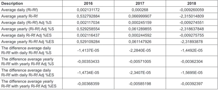
The average return before and after the adjustment uses proportional quoted half-spread (%S) and proportional effective half-spread (% ES) are not much different. The low return difference before and after the adjustment was due to low trade friction, so the low trade friction on the Indonesian capital market had an insignificant change in returns.
Table 1: Trading Friction
Year Friction
%S %ES
2018 0.0105329 0.0117679
2017 0.0117449 0.0121278
2016 0.011435 0.0114851
Difference (2018-2017) (0.001212) (0.000360)
Difference (2018-2016) (0.000902) 0.000283
Table 2: Average risk premium before and after adjustment
Description 2016 2017 2018
Average daily (Ri-Rf) 0,002131172 0,000268 -0,009260059
Average yearly Ri-Rf 0,532792884 0,066999907 -2,315014809
Average daily (Ri-Rf) Adj %S 0,002117034 0,000245159 -0,009274551
Average yearly (Ri-Rf) Adj %S 0,529258554 0,061289855 -2,318637848
Average daily Ri-Rf Adj %ES 0,002116437 0,000244592 -0,009275755
Average yearly Ri-Rf Adj %ES 0,529109284 0,061147926 -2,31893878
The difference average daily
Ri-Rf with daily Ri-Rf Adj %S -1,4137E-05 -2,2840E-05 -1,4492E-05
The difference average yearly
Ri-Rf with yearly Ri-Rf Adj %S -0,00353433 -0,00571005 -0,00362304
The difference average daily
Ri-Rf with daily Ri-Rf Adj %ES -1,4734E-05 -2,3407E-05 -1,5695E-05
The difference average yearly
Ri-Rf with yearly Ri-Rf Adj %ES -0,00368359 -0,00585198 -0,00392397
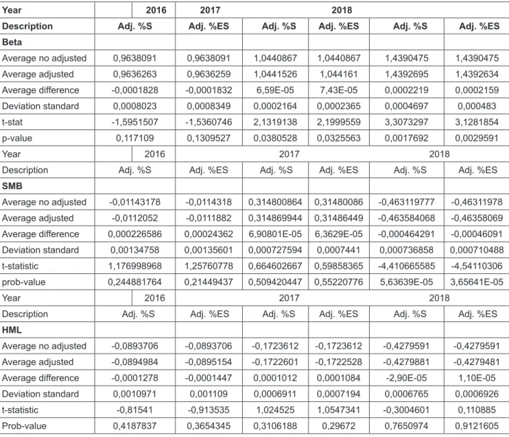
In all observation periods, all the slopes of beta or risk premium (β) were positive and significant. The test results showed that beta has a positive relation with expected return and significant both before and after adjustment. It can be concluded, based on the results of the test, that there is positive relationship between beta (β), with the average expected return as postulated in hypothesis 1 proven and significant at α 10% in 2016, 5% in 2017 and 1% in the year 2018. Nevertheless, the average beta difference that reflects market risk is able to explain the existence of trade friction. The average beta stock difference after adjustment is lower than before adjustment, with p value significant at α 10%. In 2017, the average difference in beta after adjustment to %S is 0.0000659 and after adjustment to
%ES is 0.0000743 and significant at α 5%. The average difference in beta stocks in 2018 after adjustment to %S and %ES is 0.00022 with the p value is significant at α 1%.
The low beta (β) difference after adjusment is due to the low return after trading friction. The lower the return the lower the market beta. As with noise, trade friction reflects systematic risk not idiosyncratic risk.
Noise, although not visible, can move the market and even cause the stock price to differ from its fundamental valuation (Jagadeesh & Titman, 1995). The average difference between the SMB after and before adjustment and HML before and after adjustment is quite low in all observation periods and cannot explain the return because the parameters are insignificant.
Table 3: Average difference of Beta (β)
Year 2016 2017 2018
Description Adj. %S Adj. %ES Adj. %S Adj. %ES Adj. %S Adj. %ES
Beta
Average no adjusted 0,9638091 0,9638091 1,0440867 1,0440867 1,4390475 1,4390475
Average adjusted 0,9636263 0,9636259 1,0441526 1,044161 1,4392695 1,4392634
Average difference -0,0001828 -0,0001832 6,59E-05 7,43E-05 0,0002219 0,0002159
Deviation standard 0,0008023 0,0008349 0,0002164 0,0002365 0,0004697 0,000483
t-stat -1,5951507 -1,5360746 2,1319138 2,1999559 3,3073297 3,1281854
p-value 0,117109 0,1309527 0,0380528 0,0325563 0,0017692 0,0029591
Year 2016 2017 2018
Description Adj. %S Adj. %ES Adj. %S Adj. %ES Adj. %S Adj. %ES
SMB
Average no adjusted -0,01143178 -0,0114318 0,314800864 0,31480086 -0,463119777 -0,46311978 Average adjusted -0,0112052 -0,0111882 0,314869944 0,31486449 -0,463584068 -0,46358069 Average difference 0,000226586 0,00024362 6,90801E-05 6,3629E-05 -0,000464291 -0,00046091 Deviation standard 0,00134758 0,00135601 0,000727594 0,0007441 0,000736858 0,000710488 t-statistic 1,176998968 1,25760778 0,664602667 0,59858365 -4,410665585 -4,54110306 prob-value 0,244881764 0,21449437 0,509420447 0,55220776 5,63639E-05 3,65641E-05 Year 2016 2017 2018
Description Adj. %S Adj. %ES Adj. %S Adj. %ES Adj. %S Adj. %ES
HML
Average no adjusted -0,0893706 -0,0893706 -0,1723612 -0,1723612 -0,4279591 -0,4279591 Average adjusted -0,0894984 -0,0895154 -0,1722601 -0,1722528 -0,4279881 -0,4279481 Average difference -0,0001278 -0,0001447 0,0001012 0,0001084 -2,90E-05 1,10E-05
Deviation standard 0,0010971 0,001109 0,0006911 0,0007194 0,0006765 0,0006926
t-statistic -0,81541 -0,913535 1,024525 1,0547341 -0,3004601 0,110885
Prob-value 0,4187837 0,3654345 0,3106188 0,29672 0,7650974 0,9121605
5. Conclusion
This research has developed three-factor models by loosening the assumptions of frictionless, riskless and perfect capital markets. Friction is used as a proxy for transaction costs adjusted in three-factor model as a variable that will reduce individual returns (proportional loss). This new measure of asset pricing, namely, friction-adjusted three- factor model has been tested. Using the intraday data with high frequency in the Indonesian Stock Exchange proves that the average return before and after the adjustment uses proportional quoted half-spread (%S) and proportional effective half-spread (% ES) are not much different. The indifferent returns before and after the adjustment was due to low trading friction. The estimation result of expected return on three-factor model that considers the trading friction may explain the positive correlation between expected return with beta (β), SMB (γ) and HML (δ) of entire period of observation. Trading friction causes an increase in beta (β), while SMB and HML variables cannot explain the impact of trade friction because the parameters are insignificant.
References
Acharya, V., & Pedersen, L. (2005). Asset pricing with liquidity risk. Journal of Financial Economics, 77(2), 375-410. https://
doi.org/10.1016/j.jfineco.2004.06.007
Amihud, Y., Mendelson, H., Amihud, Y., & Mendelson, H. (1986).
Asset pricing and the bid-ask spread. Journal of Financial Economics, 17(2), 223-249.
Amihud, Y., Mendelson, H., & Pedersen, L. H. (2006). Liquidity and asset prices. Foundations and Trends in Finance, 1(4), 269- 364.
Bian, G., McAleer, M., & Wong, W. (2013). Robust estimation and forecasting of the Capital Asset Pricing Model.
Annals of Financial Economics, 8(2), 1-18 Doi: 10.1142/
S2010495213500073
Cai, C. X., Hillier, D., Hudson, R., & Keasey, K. (2008). Trading Frictions and Market Structure: An Empirical Analysis. Journal of Business Finance & Accounting, 35(3-4), 563-579. https://
doi.org/10.1111/j.1468-5957.2008.02076.x
Chowdhry, B., & Nanda, V. (1991). Multimarket Trading and Market Liquidity. The Review of Financial Studies, 4(3), 483- 511.
Constantinides, G. M. (1986). Capital Market Equillibrium with Transaction Cost. The Journal of Political Economy, 94(4), 842-862.
Demsetz, H. (1968). The Cost of Transacting. The Quarterly Journal of Economics, 82(1), 33-53.
Elton, E. J., Gruber, M. J., Brown, S. J., & Goetzmann, W. N.
(2010). Modern Portfolio Theory and Investment Analysis.
Hoboken, NJ: John Wiley & Sons.
Endri, E., Abidin, Z., Simanjuntak, P, T., & Nurhayati, I. (2020).
Indonesian Stock Market Volatility: GARCH Model.
Montenegrin Journal of Economics, 16(2), 7-17. DOI:
10.14254/1800-5845/2020.16-2.1
Fabozzi, F. J., Focardi S. M., & Kolm P. N. (2010). Quantitative Equity Investing. Hoboken, NJ: John Wiley & Sons.
Fama, E. F., & Kenneth R. F. (2015). A Five-Factor Asset Pricing Model. Journal of Financial Economics, 15(1), 1-22
Fama, E. F., & French, K. R. (1996). Fama_French_multifactor_
explanations.pdf. Journal of Finance, 51(1), 55-84.
Fama, E. F., & French, K. R. (2004). The capital asset pricing model:
Theory and evidence. The Journal of Economic Perspectives, 18(3), 25-46.
Fama, E. F., & MacBeth, J. D. (1973). Risk, Return, and Equilibrium:
Empirical Tests. Journal of Political Economy, 81(3), 607-636.
Fama, E., & French, K. (1993). Common risk factors in the returns on stocks and bonds. Journal of Financial Economics, 33(1), 3-56.
Fatmawati,. Tanjung, H., & Endri. (2020). Effect of Market Risk Premium and Exchange Rate on the Return of Jakarta Islamic Index. Global Journal of Management and Business Research:
B Economics and Commerce, 5(1), 2020, 1-10.
Garleanu, N., & Pedersen L. (2013). Dynamic Trading with Predictable Returns and Transaction Costs. The Journal of Finance 68, 2309-2340.
Glosten, L.R., & Harris, L.E. (1988). Estimating the components of the bid/ask spread. Journal of Financial Economics, 21, 123-142.
Glosten, L. R., & Harris, L. E. (1988). Estimating The Components of Bid/Ask Spread, Journal of Financial Economics, 21(1), 123-142. https://doi.org/10.1016/0304-405X(88)90034-7 Huang, Y.C. (2013). Determinants of Trading Costs. In: H. K. Baker,
& H. Kiymaz, (Ed.), Market Microstructure in Emerging and Developed Markets (p. 233-252). Hoboken, NJ: John Wiley &
Sons.
Jegadeesh, N., & Titman, S. (1995). Overreaction, Delayed Reaction, and Contrarian Profits. The Review of Financial Studies, 8(4), 973-993. https://doi.org/10.1093/rfs/8.4.973 Khudoykulov, K., Rustam, A. S., & Khalikov, U. (2016) The
relationship between the risk of the asset and its expected rate of return: a case of stock exchange market of five European countries. International Journal of Modelling and Simulation, 36(4), 107-119, DOI: 10.1080/02286203.2016.1189388 Lee, S., & Upneja, A. (2008). Is Capital Asset Pricing Model
(CAPM) the best way to estimate cost‐of‐equity for the lodging industry? International Journal of Contemporary Hospitality Management, 20(2), 172-185. https://doi.
org/10.1108/09596110810852159.
Liammukda, A., Khamkong, M., Saenchan, L., & Hongsakulvasu, N. (2020). The Time-Varying Coefficient Fama - French Five Factor Model: A Case Study in the Return of Japan Portfolios.
Journal of Asian Finance, Economics and Business, 7(10), 513-521. doi:10.13106/jafeb.2020.vol7.no10.513.
Lucas, R. E. (1978). Asset Prices in an Exchange Economy, Econometrica, 46 (6), 1429-1445.
Markowitz, H. (1952). Portfolio selection. The Journal of Finance, 7(1), 77–91.
Merton, R. (1973). An Intertemporal Capital Asset Pricing Model.
Econometrica, 41(5), 867-87.
Morgenstern, O., & Neumann, J. Von. (1944). Theory and Economic. Princeton University Press.
Nguyen, C. T., & Nguyen, M. H. (2019). Modeling Stock Price Volatility: Empirical Evidence from the Ho Chi Minh City Stock Exchange in Vietnam. Journal of Asian Finance, Economics and Business, 6(3), 19-26. doi:10.13106/jafeb.2019.vol6.no3.19.
Pojanavatee, S. (2020). Tests of a Four-Factor Asset Pricing Model:
The Stock Exchange of Thailand. Journal of Asian Finance,
Economics and Business, 7(9), 117-123. doi:10.13106/
jafeb.2020.vol7.no9.117.
Razak, A., Nurfitriana, F. V., Wana, D., Ramli, R., Umar, I., &
Endri, E. (2020). The Effects of Financial Performance on Stock Returns: Evidence of Machine and Heavy Equipment Companies in Indonesia. Research in World Economy, 11(6), 131-138. doi:10.5430/rwe.v11n6p131.
Ross, S. (1976). The arbitrage theory of capital asset pricing.
Journal of Economic Theory, 13(3), 341-360.
Sharpe, W. F. (1964). Capital Asset Prices: A Theory of Market Equilibrium under Conditions of Risk. The Journal of Finance, 19(3), 425. https://doi.org/10.2307/2977928
Stoll, H. R. (2000). Presidential Address: Friction. The Journal of Finance, 55(4), 1479-1514. https://doi.org/10.1111/0022- 1082.00259