ORIGINAL ARTICLE
Three-Dimensional Numerical Simulation of Intrusive Density Currents
Sangdo An*
Korea Water Resources Corporation, 200, Sintanjin-ro, Daedeok-gu, Daejeon 306-711, Korea
Abstract
Density currents have been easily observed in environmental flows, for instance turbidity currents and pollutant plumes in the oceans and rivers. In this study, we explored the propagation dynamics of density currents using the FLOW-3D computational fluid dynamics code. The renormalization group (RNG) scheme, a turbulence numerical technique, is employed in a Reynold-averaged Navier-Stokes framework (RANS). The numerical simulations focused on two different types of intrusive density flows: (1) propagating into a two-layer ambient fluid; (2) propagating into a linearly stratified fluid. In the study of intrusive density flows into a two-layer ambient fluid, intrusive speeds were compared with laboratory experiments and analytical solutions. The numerical model shows good quantitative agreement for predicting propagation speed of the density currents. We also numerically reproduced the effect of the ratio of current depth to the overall depth of fluid. The numerical model provided excellent agreement with the analytical values. It was also clearly demonstrated that RNG scheme within RANS framework is able to accurately simulate the dynamics of density currents. Simulations intruding into a continuously stratified fluid with the various buoyancy frequencies are carried out. These simulations demonstrate that three different propagation patterns can be developed according to the value of : (1) underflows developed with ; (2) overflows developed when ; (3) intrusive interflow occurred with the condition of
.
Key words : Density currents, Environmental flows, Computational Fluid Dynamics (CFD), FLOW-3D
1. Introduction1)
Density currents intruding into water bodies most often occur in nature. Oil plumes in the oceans and highly turbid water intrusions in a reservoir are good examples of density currents. The dynamics of density currents play an important role in introducing pollutants into the water bodies which can be formed continually or can be marked by a denser fluid layer beneath a less dense fluid layer resulting in the sharp
interface of these two layers referred to as an ambient two-layered fluid system. Thus, an understanding of their dynamics and prediction of their propagation speeds are very crucial for managing water quality.
Many studies have investigated various aspects of constant-volume density currents (also known as
“gravity currents” or “buoyancy-driven currents”) using lock-exchange experiments, where a constant volume of dense fluid is released into a less dense ambient fluid. The difference in density can be
Received 26 June, 2014; Revised 15 July, 2014;
Accepted 15 July, 2014
*Corresponding author : Sangdo An Ph.D., Korea Water Resources Corporation, Daejeon 306-711, Korea
Phone: +82-51-200-2522 E-mail: [email protected]
ⓒ The Korean Environmental Sciences Society. All rights reserved.
This is an Open-Access article distributed under the terms of the Creative Commons Attribution Non-Commercial License (http://
creativecommons.org/licenses/by-nc/3.0) which permits unrestricted non-commercial use, distribution, and reproduction in any medium, provided the original work is properly cited.
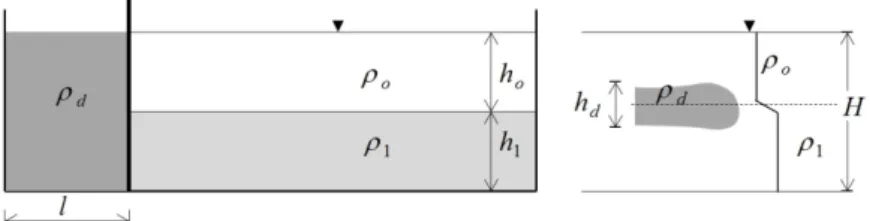
Fig. 2. Setup and definition of parameters for experiments on a density current intruding stratified fluid.
(a) Unstratified ambient fluid (b) Stratified ambient fluid Fig. 3. Sketch of density variation in a uniform and stratified ambient fluid.
generally created by adjusting the temperature or adding salt. In particular, some researchers have applied lock-exchange experiments to create turbidity currents by adding suspended particles. Density currents generally form due to a density difference between a lock fluid and ambient water.
In such a case, the density current will propagate along the bottom surface (Fig. 1). The experiments of Keulegan (1957) proposed that initial velocity would be given by ′ , where is the propagation speed of a density current, ′ is the reduced gravity defined as ′ , and is the total water depth in a tank (Fig. 1).
Fig. 1. Sketch of lock-exchange experiment for density currents propagating into an unstratified fluid.
If the density of the lock fluid is equal to the average of the densities of the two ambient fluids,
which are a two-layered fluid system (Fig. 2), the density current will intrude along the interface between the upper and the lower fluid layers and is commonly referred to an Intrusive Density Current (hereafter called IDC). Benjamin (1968) developed the theory of a density current entering a homogeneous fluid with a perfect fluid theory without considering mixing between the fluids. Thus, when a density current intrudes into the interface of a two-layer fluid symmetrically, one half of current depth ′
and one half of total depth′ can be used to obtain the propagation speed of the density current.
If an ambient fluid is stably stratified, the density stratification is described by the profile as shown in Fig. 3.
Considering density currents propagating in a stratified ambient fluid, the density currents will oscillate in simple harmonic with angular frequency (Turner, 1979) defined with
referred to Brunt-Väisälä frequency or simply the buoyancy frequency. This study aims to explore the dynamics of density currents with both unstratified and stratified ambient fluids using the 3-D non-hydrostatic FLOW-3D CFD code (Flow-3D,
2007). It is well known that hydrostatic simulation cannot reproduce the propagation speed and the formation of density currents (Fringer et al., 2006)
For turbulence modeling, the RANS approach with a turbulence model is mainly employed to simulate the density currents. In order to use experimental data for the validation and calibration of the numerical model, simulations were performed under the identical conditions that corresponds to the laboratory experimental setup in some of the published papers.
A series of numerical simulations were performed to identify the effects of some parameters on the propagation speed of density currents. The numerical simulations were focused on two different types of IDC: (1) IDC intruding into a two-layer fluid; and (2) IDC intruding into a continuously stratified fluid. The simulation results of IDC intruding into a two-layer fluid were compared with the experimental measurements from Britter and Simpson (1981).
2. Numerical methodology
2.1. Overview of FLOW-3D code
Computational Fluid Dynamics (CFD) has been widely applied in the various engineering branches of fluid mechanics due to its high accuracy. However, the application of the CFD model to the research for density currents in a stratified ambient water body is a relatively difficult challenge because the hydrodynamics of density currents propagating into a stratified ambient water body is very complex and numerically expensive to simulate. In this study, three-dimensional computational fluid dynamic simulations were obtained with a CFD code (FLOW-3D) which is a commercial code capable of fluid-boundary tracking and resolves fluid-fluid and fluid-air interfaces using its grid systems (a fixed, Eulerian approach, and structured, well ordered by a rectangular cell mesh). The model provides the transient, 3-D numerical solutions to multi-scale,
multi-physics flow problems, especially showing the capabilities for accurately simulating multi-interface flows with the improved Volume of Fluid (VOF) technique (Hirt and Nichols 1981).
2.2. Governing equations
The model simultaneously solves the governing equations for three-dimensional motion of fluids, the conservation of mass, and the transport of scalar variables. The governing equations solved with FLOW-3D are: (1) the 3-D Reynolds-averaged Navier-Stokes (RANS) equations for fluid flow with the Boussinesq approximation; (2) the continuity equation; and (3) the transport equations for each scalar variable.
r r i j i j i j i r j i j i
ρ ρ g ρ u x u ν u x x
p ρ x u u t
u
1 ' '
Equation (1) where mean velocity components (i.e., , ,
in a Cartesian coordinate system); Cartesian space ; ′′ Reynolds stress; reference density; gravitational acceleration components in each direction; kinematic viscosity; and density of density currents, which should be determined as a function of temperature and sediment concentration. Continuity equation is defined as:
0
i i
x u
Equation (2) A scalar equation can be used to compute advection, diffusion, and dispersion of scalars, defined as
u'φ'
x Γ φ φ x x u t φ
i i i i
i Equation (3)
Case # H (cm)
(cm)
(cm)
(cm)
(kg/㎥)
(kg/㎥) ′
1 20 0.04 500 50
1019.9 999.8 0.197
2 20 0.10 500 50
3 20 0.14 500 50
4 20 0.18 500 50
5 20 0.20 500 50
6 20 0.30 500 50
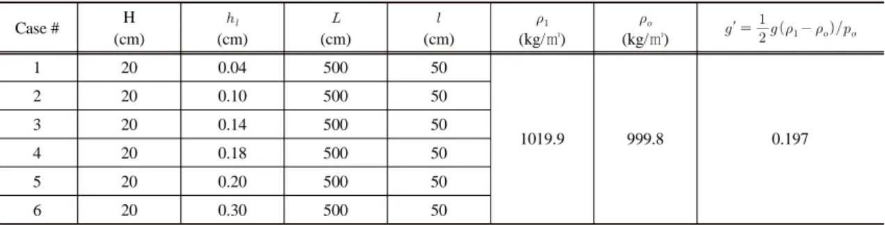
Table 1. Simulation conditions for IDC into a two-layer fluid
Fig. 4. Sketch of IDC into a two-layer fluid. Initial conditions were set up to correspond to the experiment of Britter and Simpson (1981).
where diffusivity for property ; mean scalar; ′ the corresponding fluctuating scalar; and the overbar (-) indicates averaging of fluctuating quantities. Equation (3) is a scalar equation which can solve scalar transport such as concentration and is coupled with the Navier-Stokes equations only in the buoyancy term due to Boussinesq approximation.
The FLOW-3D model includes several turbulence closure schemes, including a standard model, renormalization-group (RNG) model. In this study, we employed the renormalization group (RNG) closure scheme (Yakhot et al., 1992).
RNG closure scheme successfully captured the dynamics of density currents and showed any considerable discrepancies between RNG and LES closure schemes (An et al., 2012).
3. Problem configuration and simulation cases The comparison with the experimental measurements from Britter and Simpson (1981) and Bolster et al.
(2008) was carried out and used for the validation of
the numerical model, simulations performed under equal conditions to the laboratory experimental setup.
3.1. IDC into a two-layer fluid
In order to simulate IDC into a two-layer fluid, we arranged dimensions and initial conditions, which correspond to the experimental setup in Britter and Simpson (1981) as shown in Fig. 4. Britter and Simpson (1981) showed that the propagation speed of a density current was sensitive to the ratio of current depth to the overall depth of fluid.
This study contains various simulation cases to confirm the effect of the ratio of current depth to overall fluid depth on propagation speed. A thinner or thicker intrusive density current was obtained by changing the initial fluid depth filled behind the lock gate. Table 1 shows the conditions for this simulation setup.
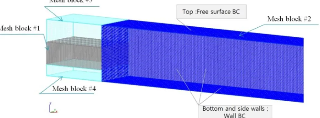
The computational domain and grids with the imposed boundary conditions are shown in Fig. 5.
The grid size in the mesh block #1 was chosen to be 7.5 mm, 10 mm and 1.25 in the in the X, Y, and Z
Fig. 5. Computational domain depicting the boundary conditions and grids for the simulations equal to the experimental setup of Britter and Simpson (1981).
directions, respectively. However, the grid size became coarser for other domains due to the memory limitation on a 32-bit operating system. Four mesh blocks were set up. The first mesh block represents a domain filled with the different fluid behind the lock gate. The second mesh block is a larger domain that contains a two-layer fluid. At the wall boundaries, wall shear stresses were modeled by defining a zero tangential velocity on solid surfaces. At the free surface, no flux conditions were imposed. For tracking the free surface, we used the fluid interfaces tracking method (i.e., unsplit and split Lagrangian methods).
For initial conditions in the numerical simulations, the velocity was set to zero and the density difference for each simulation was developed by adjusting temperature and adding concentration. Using the volumetric concentration , the mixture density of the density currents is determined by Equation
, where water temperature ℃; water density at the temperature computed by empirical formula from Gill (1982); mixture density; the specific density of a sediment particle; and volumetric sediment concentration. Benjamin (1968) suggested that for energy-conserving flows, ′ .
Benjamin (1968) investigated the value of based on inviscid-fluid theory. He showed the importance of the fractional depth . Considering the energy-conserving flow, he obtained the formula predicting the propagation velocity as a function of the fractional depth, .
2 / 1
) (
) 2 )(
(
'
d d d d
d
h H H
h H h H h g C U
Equation (4) The maximum value of is given when the approaches zero. On the other hand, the value of decreases with increasing the . When the is 0.5, approaches . The value of ranges from to when the increases from 0 to 0.5.
3.2. IDC into a stratified fluid
In this section, we consider intrusive density currents, propagating into a continuously stratified fluid, as frequently observed in nature (e.g., a reservoir, ocean, and river). The theoretical descriptions based on mass, momentum, and energy conservation were found in Cheong et al. (2006) and Bolster et al. (2008). We compared the numerical simulations with theoretically predicted values and experimental measurements in Bolster et al. (2008).
Case #
(㎏/㎥) (㎏/㎥) (㎏/㎥) (㎏/㎥) (㎏/㎥) (㎏/㎥) Note
7 0.145 1017.07 1011.49
=20cm
8 0.250 1014.86 1010.94
9 0.500 999.28 1019.96 1009.62 1019.96 1012.21 1009.63
10 0.750 1004.38 1008.33
11 0.855 1002.17 1007.78
12 1.000 999.28 1007.06
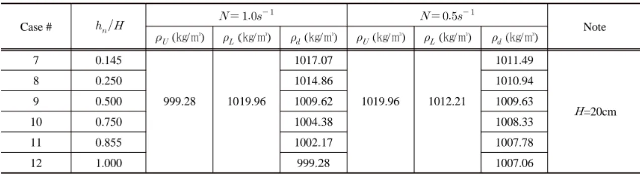
Table 2. Summary of the simulation setup for IDC into a stratified fluid
Fig. 6. Sketch of lock-exchange experiment for IDC into a stratified ambient water body. The density of the density current is determined to be where the neutral level is at .
In order to simulate an intrusive current into a stratified fluid, we arranged dimensions and initial conditions, which corresponded to the experimental setup in Bolster et al. (2008). The dimensions are 182 cm long, 23 cm wide and 30 cm deep. The total fluid depth () is 20 cm. The lock gate is positioned at 30 cm forward from the right wall (Fig. 6).
The two different stratification gradients ( ,
) are employed to evaluate the effect of the ambient water’s stratification on the propagation speed of a density current as shown Fig. 7.
When the lock gate is opened, the fluid of density beyond lock gate will propagate along its level of neutral buoyancy , where . We selected a total of 6 simulation cases and defined the different simulation setups using the parameters and . Table 2 shows the initial conditions for all the simulations. The densities of density currents for each simulation case are developed using a concentration.
Fig. 7. The density stratifications for the simulation set-up.
The density stratification is determined to be and , respectively.
4. Results and discussion
In this section, the simulation results from the cases (case 1 through 6, shown in Table 1) are explained. Numerical simulations show changes in IDC dynamics in response to changes in the ratio of current depth to overall fluid depth. After that,
second simulation results from the cases (case 7 through 12, shown in Table 2) are summarized.
4.1. IDC into a two-layer fluid
One of our interests is to find the relationship between the propagation speed and the depth of a density current, because it is easier to set up a real-time field monitoring system for the measurements of the depth rather than velocity of density currents. Then, we can calculate the propagation speed of density currents approximately using an empirical equation. Keulegan (1957) described the motion of a density current with only the depth of density current and excess density between the current and ambient fluid. He suggested the empirical equation for predicting the propagation speed of a density current through many experiments on the density current propagating along a horizontal floor into fresh water. The empirical equation was derived from the experiments undertaken mainly based on the density currents occupying approximately 1/5 of total depth (i.e., = 0.2, where is the thickness of a density current). Britter and Simpson (1981) extended the value of in the range of 1/3 to 1/10. They found that the propagation speed of a density current was sensitive to the ratio of current depth to the overall depth of fluid.
In this simulation, we demonstrated the effect of the ratio of current depth to the overall depth of fluid.
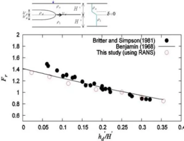
The ratio had the range from 0.045 to 0.3. The height of the interface of two fluid layers was chosen to be sharp. The range of a density current depth varied when adjusting the initial condition. The detailed simulation setup is shown in Table 2. The dimensionless parameter, densimetric Froude number, is used to show the influence of the ratio of current depth and total water depth on the propagation speed of the density current. The densimetric Froude number of an intrusive density is
given by
''
' ' H
f h h g
F U d
d r d
Equation (5) where ′ . If density currents intrude into the interface of a two-layer fluid symmetrically, one half of current depth ′ and one half of total depth ′ can be used to obtain the value of the Froude number. The variation of the Froude number () with the ratio of a current depth and total water depth is shown in Fig. 8. We observed that the Froude number varied considerably with the changes of ′′. The simulation results were plotted with experiments of Britter and Simpson (1981) and the analytical solutions from Benjamin (1968).
Fig. 8. Variation of Froude number with fractional depth.
We found simulation results showing good agreement with the theoretical curve from Benjamin’s analytical solutions and laboratory experiments of Britter and Simpson (1981).
Especially, the numerical results are more similar to the analytical values suggested by Benjamin (1968).
Decreasing Froude number with increasing the value of ′′ was observed in these simulations.
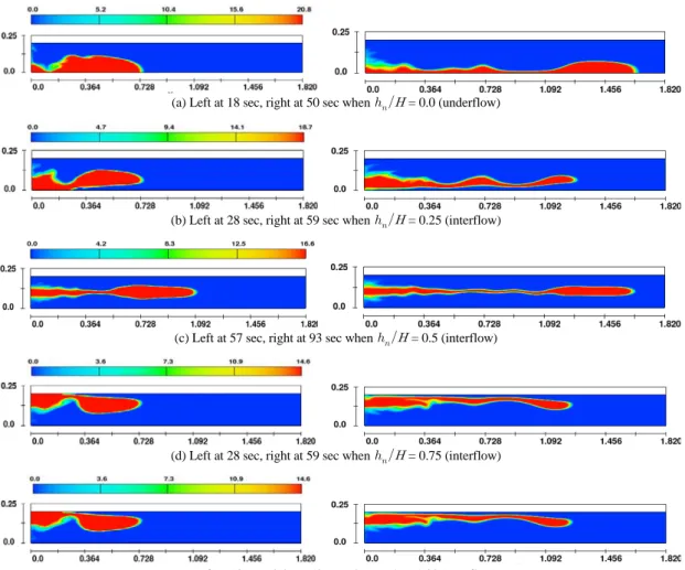
(a) Left at 18 sec, right at 50 sec when = 0.0 (underflow)
(b) Left at 28 sec, right at 59 sec when = 0.25 (interflow)
(c) Left at 57 sec, right at 93 sec when = 0.5 (interflow)
(d) Left at 28 sec, right at 59 sec when = 0.75 (interflow)
(e) Left at 18 sec, right at 50 sec when Hn/H= 1.00 (overflow)
Fig. 9. Temporal evolution of the intrusive density currents into a stratified ambient fluid where the density of fluid behind lock gate was created using concentration. Density currents showing temporal evolutions were shown by the concentration contour.
4.2. IDC into a stratified fluid
In a uniformly stratified fluid, Maxworthy et al.
(2002) predicted that a density current would travel at a constant speed () which took the form,
. Maxworthy et al. (2002) and Ungarish (2006) experimentally determined the values of equal to 0.266 and 0.25, respectively, by experiments.
Bolster et al. (2008) carried out extensive experiments to determine how the propagation speed of density currents depended on the variation of density of density currents (or ). They suggested an analytical solution for determining the propagation speed using
the assumption that a perfect conversion of energy occurs between the kinetic energy and potential energy as the density field adjusts.
1 2 12
1 21 2
H
H FNH h
Ud n
Equation (6) We simulated density currents intruding into a continuously stratified fluid with the buoyancy frequency ( , ). The numerical simulations were conducted for density currents propagating into a continuously stratified fluid over the entire range,
≦ ≦ ( Fig. 9).
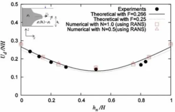
The propagation speed of numerical results and experiments are shown and compared to the theoretical calculations in Fig. 10. They show good agreements with theoretical curves calculated by the energy model in Bolster et al. (2008).
Fig. 10. Comparison of dimensionless intrusion propagation speed for numerical simulations (□, N=
1s-1; ∆, N=0.5s-1) and experiments (●, from Bolster et al. 2008). The line and dashed line are the predictions by the energy model in Bolster et al.
(2008).
In numerical simulations, we observed that the density current propagated slower when the current traveled at mid-depth, while maximum speed occurred when it traveled either at the top or bottom.
5. Conclusions
In this study, we explored the propagation dynamics of intrusive density currents using a three-dimensional, non-hydrostatic numerical model.
The numerical simulations focused on two different types of IDC into a two-layer ambient fluid and a linearly stratified fluid. In the study of IDC into a two-layer ambient fluid, intrusive speeds were compared with laboratory experiments and analytical solutions. The numerical model showed good quantitative agreement for predicting propagation speed of the density currents. We also numerically reproduced the effect of the ratio of current depth to
the overall depth of fluid. The numerical model provided excellent agreement with the analytical values suggested by Benjamin (1968). It was also clearly demonstrated that RNG scheme within RANS framework was able to accurately simulate the dynamics of density currents. It indeed indicates that this technique is valid for field scale applications with fast computational times without significant loss in performance. We simulated density currents intruding into a continuously stratified fluid with the various buoyancy frequencies. Numerical simulations captured very well the formation of internal waves and evolution of density currents in response to the ratio of to . The propagation patterns can be classified into three regimes: (1) underflows developed with ; (2) overflows developed when ; (3) intrusive interflow occurred with the condition of . Extension of this study in ongoing to investigate pollutant transport by density currents in a stratified ambient water body.
References
An, S. D., Julien, P. Y., Venayagamoorthy, S. K., 2012, Numerical simulation of particle-driven gravity currents, Environ. Fluid Mech., 12(6), 495-513.
Benjamin, T. B., 1968, Gravity currents and related phenomena, J. Fluid Mech., 31(2), 209-248.
Bolster, D., Hang, A., Linden, P., 2008, The front speed of intrusions into a continuously stratified medium, J. Fluid Mech., 594, 369-377.
Britter, R. E., Simpson, J. E., 1981, A note on the structure of the head of an intrusive gravity current, J. Fluid Mech., 112, 459-466.
Cheong, H. B., Kuenen, J. J. P., Linden, P.F., 2006, The front speed of intrusive gravity currents, J. Fluid Mech., 552, 1-11.
FLOW-3D, 2007, User guide and manual release 9.3, Flow Science Inc, Santa Fe, NM.
Fringer, O. B., Gerritsen, M. G., Street, R. L., 2006, An unstructured-grid, finite-volume, nonhydrostatic, parallel coastal ocean simulator, Ocean Modell.,
14, 139-173.
Gill, A. E., 1982, Atmosphere-ocean dynamics.
Philosophical transactions. Series A, mathematical, physical, and engineering sciences, Academic Press, New York.
Hirt, C. W., Nichols, B. D., 1981, Volume of fluid (VOF) method for the dynamics of free boundaries, J. Comput. Phys., 39, 1-11.
Keulegan, G. H., 1957, Thirteenth progress report on model laws for density currents an experimental study of the motion of saline water from locks into fresh water channels, U. S. Natl. Bur. Standards Rept. 5168.
Maxworthy, T., Leilich, J., Simpson, J., 2002, The
propagation of a gravity current into a linearly stratified fluid, J. Fluid Mech., 453, 371-394.
Turner, J., 1979, Buoyancy effects in fluids. Cambridge University Press, New York.
Ungarish, M., 2006, On gravity currents in a linearly stratified ambient: A generalization of Benjamin's steady-state propagation results, J. Fluid Mech., 548, 49-68.
Yakhot, V., Orszag, S. A., Thangam, S., Gatski, T. B., and Speziale, C. G. 1992. “Development of turbulence models for shear flows by a double expansion technique.” Phys. of Fluids, 4, 1510-1520.