Identification of the Moving Noise Source in a Circular Sawblade by the Experimental Acoustic Intensity Technique

82

Identification of the Moving Noise Source in a Circular Sawblade by the Experimental Acoustic Intensity Technique

음향인텐시티법에 의한 원형 톱날에서의 이동소음원 규명

Jae Eung OH* Dong Kyu Kim, Bum S니ng Ha? Sun Hy Won**

오 재 응f 김 동 규, 하 범 성, 원 선 희**

ABSTRACT

This study investigates the feasibility of identifying aero-acoustic source occurring with rotating sawblade. The acoustic intensity technique takes useful advantage of 3 D, intensity vector flow and contour plots. The estimations of the near field behavior and the frequency domain vector or scalar acoustic intensity are measurement used for source identification purposes. According to the results, the turbulence produces in the vicinity of teeth of circ^니lar sawblade. The evidence of the influence of the vortex stmeture on the fluctuating sawblade pressure measurement is derived from the measured acoustic intensity. As the rotating speed increases, the interaction can be a significant source mechanism producing Dopplerphenomenon.

요 약

본 연구에서는 회전톱날에서 발생하는 공기소음원(aero^거cousticsource)규명의 실현가능성을 검토하였다. 음향인텐시 티 법은 3^{차원 선도}(3-Dplot), 인벤시티 벡터에너 지 선도(intensity vector energy flow), ^동고선도(contour plot)^{등의 표} 현에 유용한 장점 을 갖고 있다 근거 리 음장(nearfieE)거 동에 대 한 추정, 주파수영 역에 서 의 벡 터 또는 스칼라 음향인텐 시 티는 소음원규명의 목적으로 사용되는 측정기법이다. 결과에 따르면 난류 (turbulence)^{는 원형톱날의 이} (teech) ^부근에서 나타나며, 톱날의 변동압력 측정에서 와류구조의 영향에 대한 근거는 측정된 음향인텐시티에 의해 도출된다. 또한 회선속 도가 증가함에 따라, 상호작용(interaction)^{은 도플러현상}(Doppler phenomenon)일으키는 중요한 소음메타니즘이 된 수 있다.

_______________________________________________ I. Introduction

* Precision Mechanical Eng. Han Yang Univ.

**Mechanical Eng. Iowa State Univ. U. S. A.

The circular sawblade is probably the most common cutting tool in the wood industry. The

Identification of the Moving Noise Source in a Circular Sawblade by th으 Experimental Acoustic Intensity Technique 83

noise radiated by the idealing saw is excessive, and it results from a complicated mechanism. In order to seek methods of noise reduction, it is necessary to identify and rank the prominent sources of nise. If the noise sources are better understood, then the design process for reduced noise can be more useful. Traditionally, the noise source identification and rank ordering has been carried out by using the lead wrapping technique' n. near fi^이d holography⑵, an inverse computational method⑶，multi-dimensional spectral analysis tec- hniques(4), and intensity measurement methods ⑸.

Methods attemps to reduce machinerynoise ideally based on knowledge of the contribution of each individual noise to the overall radiated noise. Thus noise source identification is of vital importance for any noise reduction program, and a variety of methods have been developed in the past to serve this purpose. However, there is still a need for techniques that allow one to measure the distribution of noise sources with the operating in situ.

Preliminary work on the idling circular saw noise identification problem by Mote and Zhu-in 1980

⑹ and recently by Kimura⑺ and Singh⑻ at the University of California, Berkeley focused on the development of a phenomenological, kinematic source model and measurements of acoustic inte­ nsityin ^나lenormal, radial and tangential directions.

They assumed that source models produce a spe­

cific acoustic intensity(time-averaged energy flux) in front of the saw. The acoustic intensity method has merit for noise source identification in a multi-source steady situation. The noise characte­ ristics of individual source can be more accurately determined by near field acoustic intensity meas- urements. Recently there have been rapid develo­ pments in the techniques of measuring acoustic intensity. Of these techniques, the two closely- spaced microphone method has proven to be the

popular.

In this study, the noise sources in the radial, tangential and normal directions to the circular sawblade are discussed. The purpose of this study is to identify the prominent noise producing dire­

ctions in circular sawblade. The noise sources st^니died was a circular sawthat served asan idealiz ed mod^이 for a kinematic and dynamic dipole source.

II. Theory

2.1 Theory of Rotating Disk Acoustics Model

2.1.1 Review and Assumption

This study is primarily concerned with the feasibility of identifying aero-acoustic source (s) associated with the rotating disk including idling

soundat a discrete frequency fs will beconsidered as a schematic representation of the model as shown in Fig.l. A dipole force vector F will be assumed to be located in the vicinity of the disk edga. The emphases of the analysis are on the an alyticalestimation of typical near field behavior and on the frequency domain vector or scaler techniques used to acquire near field data for diagnostic purposes.

A source S of frequency fs is considered to be moving with subsonic velocity MS=VS/CO relative to the stationary observation point P located in the near field. First, the kinematics of the problem for both translating and rotating sources is exam­

ined :the rotating source is assumed to be in a steady angular rotation with fd Hz. The observed frequency fP is related to fs and kinematics； the sign of the intensity probe is also examined. Next, the source is taken to bea translating or rotating dipoleof oscillating force F(t). Bothstationary and moving dipole models are used to investigate the typical sound field generated by a rotating disk.

84

Fig. 1. Schemmatic diagram for acoustic source of rotating disk.

韓:國言•響學會估10谷(i號(1991)

(4) The source is modeled as an oscillating sphere of radius a : this source may be compact especially at low frequencies. i.e.ksa=2n-fs/ Co

=，r/^人 s.

(5) The source may be stationary or moving : both cases will be considered.

(6) Only the free acoustic field is considered^

(7) The measurement or observation field point P is stationary. Further it is assumed 나lat the intensity probe does not disturb the acoustic field.

The following there coordinate systemsare used :Cartesian (x,y,z) for translating sources analysis and fi^이d vector measurements, cylindrical(R. , C) for the kinematic and dynamic analysesof the rotating sources, and sphericalfor the free sound radiation study.

These models are then applied to the idling saw problem and predictions are compared with mea­

sured intensity data.

The generic rotating disk model considered in this study is applicable to the rotary cutters such as a saw, disk drives, air moving devices, andother rotating machinery. The following assumptions are made.

2.1.2 Oscillating Sphere Model

The point dipole model as given by the first two theories will be used in this report : it will also be compared with the Curie-Lighthill theory'

⑵ which has been applied to the disk acoustics problem. Chief advantage of the oscill^거ting sphere model is the prediction of neau field and its ada­ ptability t the rotating source model. A harmoni­ cally oscillating sphere of radius "a" exerting a sinusoidal force Fz exp( j - wst) in the z direction can treated as a finite harmonic dipole located at the origin, the z axis is the dipole axis. Acoustic pressure p and radial v^이ocity u for free field spherical radiation in(r,0,y) coordinates are as follows for r A ；

p(r,9,t) Fz (1+jlqr) co魚 以［g -k,(【T)|

4n r1 2 3 (1+jkg) (1) The disk rotational speed fd is constant and

subsonic, i.e. Md=Vd/C0=2^fdRd /Co< 1.

(2) The acoustic source S is a single dipole indu­

ced by the periodic vortex shedding,9"11'. Acc­

ordingly, the source is located near the edges, i.e.Rs=0(Rd).

(3) The single source may also be given by a combination of N identical but uncorrelated sources distributed around edges. The single net source could then be moved to the origin 0.

(1)

Identification of the Moving Noise Source in a Circular Sawblade by the Experimental Acoustic Intensity Technique 85

顷히) = , 产)

4KpoCo ksr3 GOS。- ks(r-a)J

1 + jksa (2)

Mean square pressure <p2>t and the resistive acoustic intensity in the radial direction Ir are :

<P2>t = Prms = ^Re[p-ri (3)

lr(r,e,cos) =}Re[0•甘]=<? 好 r；

2 z° (l+k?r2)

(4)

The resistive intensity in the q direction is zero.

The sound power W radiated at ws is given by the product of spatially averaged Ir and the rad­ iation surface area A.

W(ws) ■= <Ir>A =---미--- -

247ta호p°Cq (1 + k?a2 ) (5)

The source is a point or compact dipole if ks a« 1.

2.1.3 Acoustic Intensity of Near Hid in Disk The acoustic near field condition is given by ksr<<! or r«A,s. Accordingly, Equations(1-4) show that in the near fi시d for r^a,

D =£OS0 u =海。

r2 ， r r3

Ir = 뿐金 3 = 으 = ljkspoCor ⑹

We note that the field is very reactive as the

radiation impedance z is purely imaginary, and that the pressure and velocity gradients are very steep.

Further, Ir is not equal to<p2>r / />0C0. Also, L=^〈p

°〉/which froms the basis of far field sound source power measurements as Ir and W can be easily related to <p2>t,

2.2 Basic Theory of Acoustic Intensity

In an elasto-acoustic system, the acoustic inte­ nsity is a vector quantity defined as a product of the acoustic pressure and the corresponding particle velocity at a given point. When there is no flow, the one dimensional equation of motion is defined as follows'13'

3u(t) 3p(t) _ 0

P■耳厂3r -0 ⑺

where p is the density of air, u(t) is particle velocity in the r-direction.

the acoustic pressures pjt) and p/t) are mea­ sured at two closely-spaced points in the r-direc­

tion. The gradient of acoustic pressures is appro­

ximately represented as

3p(t) . P2(t) - Pl(t)

3r 最 ⑻

where r is the distance between two points where the acoustic pressures are measured. The approx­

imate particle velocity is

u(t)=-丄 r 鎏 dt

P / ar

J -oo

=-丄"{ P?(t) -pi(t) } dt 怎)

86 S?阈"牌學會温.1（1谷6號（1991）

and the acoustic pressure p at the center of two points can be approximated as p(t) ={p】(t)+p?

(t)}/2. Therefore the acoustic intensity I becomes

I = -lim 1. I u(t). p(t) dt = (p(t)- u(t)〉

J。。T J”

技+ {P2(0 - Pl(t)J〉

(10)

where < ^〉denotes a time average. Because the process is stationary and ergodic /p./t)dt>

becomes zero, and using the relation of

〈Pi(t)/P2(t)dt=— pjt)/p^】(t)dt^〉，the acoustic intensity of equation (10) can be rewritten as follows

I = - 一^〈 Pi(t) P2(t)血〉

pAr 丿 3 ₍₁₁₎

By computing the Fourier transform of equation (11), acoustic intensity 1(^ — ^) in frequency domain is expressed as

I (fi - f2)=——1— I 匝」G12(f)} df 2兀pAr丿n f

(12)

where Im is the imaginary part of a complex number and G12(f) is the cross spectral density function of the acoustic pressures at the two points.

Hence acoustic intensity can be determined by measuring the imaginary part of the cross-spectrum between the pressures and measured at clo­ sely -spaced points. In this paper, a 2 channel FFT

analyzer was used to compute theacoustic intensity in the frequency domain.

Hl. Experiment

3.1 Experimental Apparatus and Method

An idealized experiment seemed to offer most promise in the study of the feasibility of ^나sing acoustic intensity measurements on a circular saw.

The acoustic intensity of the moving noise source in a circular saw was measured to idemfy the source characteristics. The acoustic intensity was measured in a rectangular semi-anechoic chamber (3.3m x 2.0m x 2.3m), with a cut off frequency of about 30() Hz, as shown in Fig.2 The variable speed drive motor was located outside the to minimize its contribution to room noise, the acoustic intensity was measured in three directions at points in front of the sawblade (Fig.3). The acoustic intensity measurement surfaces were 38 mm away from the sawblade.

3.2 Measuring Systems and Data Processing Techniq^니 es

Acoustic intensity measurements were made at the predetermined grid points . The distance between the grid points was precisely kept at 5 ()mm. Two 3.2mm Rru시 & Kjacr( B&K 413K) microphones m a side-by-side configuration 13mm

Fig. 2. Schematic diagram of expsmient시 set up for noise stjurce identification of a circuku '貝

Identification of the Moving Nsse Source m a Circular Sawblade by the Exper,mental Acoustic Intensity Technique 87

Nonnal Direction 둬

Radial Direction

Tangential Direction

Fig. 3. Three Directions of Measurement for Acoustic Inte-

nsity in a CirCular Sawblade. Fig. 5. Microphone positioning system.

Fig. 4. Two microphones mounted in a cylinderical holder.

apart were used to measure the acoustic intensity (Fig.3). The microphones were mounted in cylin- drical holder as shown in Fig,4. The holder position about its axis of symmetry was controlled with 저 rotation drive, and 比。hoeder was rotated about the axis D-D to change the direction of acoustic intensity. In this experiment, the height of the measurement point was set at the height of the axis the sawblade. The height of measurement point P was adjustable. Measurement point was positioned parallel to the plane of the disk with a motor driven traverse (Fig.5). Acoustic intensity spectra were computed from cross-spectra density measurements on two-^사1am^冶 1 FFT analyzer(HP 5423A), At each measurement point 512 averages of the spectra were obtained in a 6.25 Hz bandw- idth in the frequency range 250Hz to 1600Hz. The lower and upper frequency ranges were limited by the microphone spacing, the spectra at each measuring points in each of three directions were the average of 512 spectra with the microphones positions interchanged after every 256 samplings

88 韓國普•響學會誌10卷6號（1的1）

to compensate for differences in phase between the two microphones. Each acoustic intensity, computed form this data, is the vector component of sound power in one of the three particular directions. The moving source was identified from these data. A microphone positioning system con­ trols the position of the microphone relative to the

Fig. 6.Measuring point in acircular sawbladeforverification of acoustic intensity at the sameradius in case of 25 points.

Fig. 7. Measuring point in a circular sawblade with diameter 228mm, 72 teeth and damping.

sawblade surface. The measurement points were 25 points and 49 points in front of sawblade as 아】。"】 in Fig.6 and Fig.7. In order to identify noise source mechanism, these res니Its were shown by contour, 3-D and intensity vector flow plots.

IV. Results and Considerations

4.1 Acoustic Intensity radiated from a Circular Sawblade

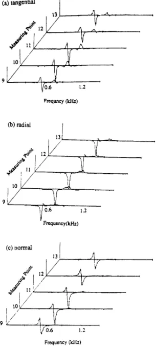
In this experiment, microphones were moved in measurement positions automatically, but it took about very long time to record the spectra inthree directions at a point. If the measured acoustic intensity spectra in tangential, radial, and normal direction■ at 900rpm were identified by the mech­

anism of radiation from the sawblade, measuring time would be saved. With same source receiver distances of tangential, radial and normal directions on the sawblade the spectra of acoustic intensity were obtainedasshown in Fig.8. This figure shows the representative waterfall plots for the same radius range and each direction of measurement on 25 points. All the spectra have the same scale with the maxima frequency. Therefore, the mea­

surement taken at one point could replace another points at the same distance to reduce measurement time. The spectra of acoustic intensity at radial and normal directions were identical to each same radius as shown in Fig.8.

4.2 Characteristics of Acoustic Intensity due to Rotating Speed

Fig.9 shows such waterfall plots of acoustic intensity at each directions of measurement taken during the variations of rotating speed. All spectra have the same scale, with the maximum height plotted equal to the value of the highest peak, whichis at the lowest runout frequency at 900rpm.

As the rotating speed incre^거sed, these response

Identification of the Moving Noise Source in a Circular Sawblade by 나le Experimental Acoustic Intensity Technique 89

Fig. 8. Waterfall plot of circular sawblade at 9CX)rpm of each direction of measurement on the same radius.

and peak frequencies of acoustic intensity also increased at the peak frequency. In the other hand, the spectra of acoustic intensity due to change of measurement of sawblade at the same rotating speed is shown in Fig.10. The level of acoustic intensity had the maximum in the vicinity of rim.

Also, the responses of acoustic intensity at each directions of measurement shows the similar cha-

Frequency (kHz)

Fig. 9. Acoustic intensity spectra for sawblade at various rotating speed.

racteristics. P'ig.ll shows the responese of acoustic intensity in each directions of measurement at same measuring points. The level of acoustic int­

ensity in tangential and normal measurements directions had values from negative positive acco­ rding to increase of the rotating speed. Specially, the response in radial direction of measurement only has positive level of acoustic intensity. The results mean that the acoustic intensity of radial direction has only source without sinking.

90 韓國件響學會誌1()卷6號(1991)

Ffcqticncy (kHz)

(c) 1500 rpni (d) 18()() 디)m

Fig. 10. Comparisons of response of「acoustic intensity due to changing ofmeasunng points at tangential dire ction of micriphone poistion.

Fig. 11. Acoustic intensity spectra of each measuring dire­

ction and rotating speed at the same measuring point (No.17),

Identification of theMoving Noise Source in a Circular Sawblade by the Experimental AcousticIntensity Technique ⁹¹ 4.3 Noise Source Ranking due to Spatial Avera­

ging of a Circular Sawblade

The use of acoustic intensity rather than sound pressure to determine sound power means that measurements can be made in situ, with steady background noise and in the near field of mach- ines. The sound power is average normal intensity over a surface enclosing the source multiplied by

Frequency (kHz)

Fig” 12. Acoustic intensity spectra for ranking source inen- tification of spatial averagingin a circular sawblade at ratating speed 900rpm.

J

(b) radial

Frequency (kHz)

Fig- 13. Acoustic intensity spectra for ranking source inen- tification of spatial averaging ina circular sawblade at ratating speed 1200rpm.

orbers of sound) are present within the surface.

After a surface has been defined, we need to spatially average the intensity values measured normal to the surface. To obtain an average int­ ensity value from each side, one of two spatial averaging techniques can be used. In this study, an intensity surface covering the measuring object is dividedup into small segments, and theacoustic intensity in each segment is measured. The results were averaging to find the source location and

韓國音響隼會誌10卷6镜(1991) 92

Fig. 14. Acoustic intensity spectra for ranking source men-

* tification ofspatial Averaging in a circular sawblade at ratating speed 1500rpm.

source ranking. Fig.12-Fig.15 show the results averaged spatial at radius rotating speeds and directions of measurement. By these results, the

Frequency (kHz)

Fig. 15. Acoustic intensity spectra for ranking source inen- tificationof spatialaveragingin a circular sawblade at ratating speed 1800rpm.

comparisons between theoretical and experimental frequenciesof moving source in a circular sawblade are shown in Table 1.

4.4 Acoustic RMiation Pattern of a Circular Sawblade by Contour and 3-D Plots Every noise control problem is first of all a problem of location and identificationof th^픈 source.

Acoustic intensity measurement offers several ways of doing this which have considerable advantages

Identification of 나le Moving Noise Source in a Circular Sawblade by the Experimental Acoustic Intensity Techni이ue 93

over previous techniques. Contour and 3-D plots give a more detail picture of the sound field generated by a source. Several sourceand or sinks can then be identified withacc^나racy. In this study, lines of equal intensity can be drawn by interpo­

lating (Cubic Spline method.) and joining up points of equal intensity. They are sometimes called iso- -intensity lines and they can be drawn either at single frequencies. A separate plot can be made for negative-going intensity which can be used to locate sinks of sound energy. The same data

can be used to generate 3-D plot which provides easy visualization of the sound field generated by a source. We can, of course, also make contour maps and 3-D plots with acoustic intensity mea­

surements. But, intensity maps can be made in the near field where the correlation between the measured intensity lev^시s and the source position is greater. Due to the change of measuring direc­

tions, the acoustic intensity is shown in all cases.

Fig.16-Fig.18 show contour maps. Specially Fig.

17 shows that the acoustic intensity had the so^니-

(a) 900 rpm (b) 1200 rpm

(d) 1800 q)ni (c) 15()0 rpm

Fig. 16- Contour plots of circular sawblade at tangential measurement direction of microphone position due to change of rotating speed.

94 韓阈片噜學會能.1()苍6號(1991)

Fig. 17. Contour plots of circular sawblade at radial measiurement direction of microphone position due to

(b) 1200 rpm

(d) 18(X) rpm

change of rotating speed.

rces in the vicinity of the rim. All figures are drawn to the same scale for comparison. The comtour maps are oriented with rotating speed toward different patterns. When the rotating speed is reduced to poorpm, several things occur. A dominant positive circle contour line appears with near the centerof sawblade at tangentialdirection of measurement. The positive contour line is tow­ ard center at tangential direction of measurement but the largest contour line is appeared at rim of

sawblade on the radial direction of measurement.

When the directions of measurement is normal, the contour is not appeared clearly except at 12 (X)rpm. Interestingly, this contour pattern is always not on the center thorugh the rotating speed but occurs on a rim.

The acoustic intensity distribution in the circular sawblade is fairly even with acoustic intensity maxima close to the center and rim. Thedominant phenomenon are appeared as the rotating speed

Identification of 나le Moving Noise Source in a Circular Sawblade by the Experimental Acoustic Intensity Technique 95

(a) 900 rpm (b) 1200 rpm

(c) 1500 rpm (d) 1800 rpm

Fig. 18. Contour plots of circular sawblade at normal mea surement direction of microphone position due to change of rotating speed.

increases. In fact, the 3-D plots of acoustic inten- sity are 아lown the pattern of source at rim (Fig.

19-Fig.21). The most case measured at radial direction(Fig.20) has acoustic intensity on the center ofsawblade. The negative value of acoustic intensity occurs at the outside from rim thorugh change of rotating speed. But, at radial measure­ ment direction the pattern of acoustic source is notappeared apparently. Therefore, the noise source is composed of moving andstationary components

uniformly distributed at the sawblade rim. The stationary component is given by a number of identical, equally spaced dipoles radiating at a discrete frequency governed by the rim shape and speed. The moving component is produced by the turbulent eddies convecting over the sawblade surface and teeth. This can be modeled via a number of identical radial dipoles rotating at a velocity bounded by the rim speed. From the results mentioned above, it can be seen that the

96 辩阈 "치!學會上 1() 谷 6 號(1991)

Fig. 19. 3 D plots of cirular sawblade at tangential direction of measuremnt due to change of rotating speed.

Fig. 20. 3“D plots of cirular sawblade at normal direction of measuremnt due to change of rotating speed

source of sawblade should have to be modeled as spherical source.

4.5 Acoustic Intensity Vector of a Circul히 Saw blade

Vectorintensity measurementshave been applied

to many problems in areas such as room acoustics, musical acoustics, diffractions, etc. Assound source with acomplicated nearfi^이d in a circular sawblade is considered, the circular sawblade was rotated toward counter clockwise with motor outside of anechoic chamber. Fig.22 shows a plot of the intensity vectors parall^이 to the sawblade, measured

Identification of the Moving Noise Scarce in a Circular Sawblade by the Experimental Ac。니Stic Intensity Technique 97

(a)900rpm

(b) 1200 rpm

Fig. 21. 3-D plots of cirular sawblade at radial direction of measuremnt due to change of rotating speed.

(c) 1500 rpm

at 49 points close to surface. Arrow length is proportional to the intensity, and it shows the direction of flow. It can be seen that the origin

98

(d)1800rpm

Fig- 22. Acoustic intensity vector flow due to rotating speed for tangential-radial plane.

(a) 900 rpm

鯨阈汚牌學會誌1()卷fi號(1991)

of te intensity flow closely matches the position of the rim in a circular sawblade and also exists on the center. It can be also seen that theacoustic intensity flows toward clockwise in spite that the rotating direction is counter clockwise. Therefore, the moving noise source is produced by the turb­ ulent eddiesconvectingover thecenter ofsawblade and teeth. Thus a vector intensity mapping of the near field makes it possible to very precisely locate the points where the intensity is entering the system and identifythe major source areas. In this vector plots, the source location has been fo^나nd nom mapping of the tangential-radial plane inte-

(b) 1200 rpm

(c) 1500 rpm

« •

■ • I *

- I

, 1'

• , r

(d) 1800 rpm

Fig. 23. Acoustic intensity vector flow d니e to rotating speed for radial-normal plane.