콘크리트의 구속효과와 재료 비선형을 고려한 콘크리트의 구속효과와 재료 비선형을 고려한 콘크리트의 구속효과와 재료 비선형을 고려한 콘크리트의 구속효과와 재료 비선형을 고려한 내부 구속 중공 기둥의 축력 모멘트 상호작용 분석 내부 구속 중공 기둥의 축력 모멘트 상호작용 분석 내부 구속 중공 기둥의 축력 모멘트 상호작용 분석 내부 구속 중공 R.CR.CR.CR.C 기둥의 축력 모멘트 상호작용 분석---- Analysis of the Axial Force-Bending Moment Interaction
for an Internally Confined Hollow R.C Column Considering the Confining Effect and the Material Nonlinearity of Concrete
한택희1) 염응준2) 윤기용3) 강진욱4) 이명섭5) 강영종6)
Han, Taek Hee Youm, Eung-Jun Yoon, Ki-Yong Kang, Jin-Ook Lee, Myeoung-Sub Kang, Young-Jong
--- ABSTRACT
Concrete in a R.C column has enhanced strength and ductility because it is confined by transverse reinforcements. But R.C columns are designed based on linear analyses by stress block method without the confining effect or the nonlinearity of the concrete.
These make the significantly difference between the analysis results and the experimental results. And also ICH R.C column(Internally Confined Hollow R.C column), a new-typed column, has enhanced moment capacity and axial strength by a settled steel tube when it is compared with a hollow R.C column. Thus in this study, nonlinear P-M interaction models for a general R.C column and an ICH R.C column were developed considering the confining effect on the concrete in a column. With the developed model, parametric studies were performed and the developed column models showed reasonable and accurate results.
--- 1. Introduction
1. Introduction 1. Introduction 1. Introduction
A column is a vertical structural member transmitting axial compressive loads, with or without moments. But the column subjected to pure axial load rarely, if ever, exists. All columns are subjected to come bending moment, which may be caused by eccentric loads or lateral loading such as from wind or earthquake. Thus it is important to predict the behavior of a column under combined load for safe design. An axial load-bending moment interaction diagram (P-M interaction diagram) is one of the most effective methods to show the behavior of columns subjected to combined loads.
1) 고려대학교 공학기술연구소 연구조교수 2) 고려대학교 강구조협동과정 박사과정 3) 선문대학교 건설공학부 교수
4) 삼성물산 주 건설부문 토목기술팀 차장( ) 5) 삼성물산 주 건설부문 토목기술팀 부장( ) 6) 고려대학교 사회환경시스템공학과 교수,
But present P-M interaction diagrams are plotted by calculating equivalent stress blocks with assumed linear stress model and the unconfined strength of the concrete. Thus this present method gives conservative results because it cannot consider the enlarged strength of the confined concrete or nonlinearity of the concrete. But concrete in a column is confined by reinforcements or a tube and it's behavior is not linear. Thus it could give more realistic results to calculate the P-M interactions considering the nonlinearity and enhanced strength of the concrete confined by transverse reinforcements. And a seismic load is one of the main lateral loads to govern the behavior or the failure of a column. To minimize the hazard to life and limb in the event of an earthquake, bridges may suffer damage but the prevention of structural collapse should be ensured. To meet this basic philosophy, two approaches are presently used to provide earthquake resistance. One is the design for ductility in the piers and the other is the design for structural isolation.
The seismic resistance of bridge structures is normally achieved by designing the piers for both strength and ductility. Generally, it is uneconomical to design a bridge pier to respond to the inertial loads induced by the design earthquake. The ductile design approach allows the piers to be designed for inertia loads somewhat smaller than the elastic inertial elastic loads induced by a severe earthquake. Thus ductile bridges piers are designed to dissipater seismic energy by the formation of plastic hinges. For a satisfactory design, checks should be made to ensure that the ductility of the plastic hinges is greater than the ductility demand under the design ground motions. To get the ductility factor of a column, moment-curvature analyses or a lateral force-lateral displacement analyses of a column are required. In this study, a nonlinear P-M interaction analysis program were developed by using the nonlinear material models developed from a prior research considering the nonlinearity of the materials. The developed column model is applicable for all types of R.C columns which have circular sections.
2. Strain Compatibility Solution 2. Strain Compatibility Solution 2. Strain Compatibility Solution 2. Strain Compatibility Solution
According to recommended methods to plot interaction diagrams of R.C columns by current specifications like ACI Code, forces and moments are calculated from assumed stress block and these methods cannot consider the material nonlinearities and the increase of the confined concrete. The generally used calculation process is illustrated in Fig. 1 for one particular strain distribution. The cross section and one assumed strain distribution are shown in Fig. 1. The maximum compressive strain ( εcu) is set 0.003, corresponding to failure of the section. The location of the neutral axis and the strain in each level of reinforcement are computed from the strain distribution.
Fig. 1 Calculation of Axial Force and Moment by Current Specifications
ε ε ε εcu
Ascfy
Strain
Cb 0.85Cb
0.85fco
Astfy
Stress Acting on Concrete
Force Acting on Rebar
In these methods, the compressive force on the concrete is computed form the assumed stress block. The stress block is assumed to have the magnitude of 85% of the unconfined concrete strength (fco) and the distributed length of the stress block is assumed to be 85% of the distance between the neutral axis and the outer surface of the column (Cb).
And the forces on the longitudinal reinforcements are computed from the stress in each layer of reinforcement. The forces in the steel layers are computed by multiplying the stressed by the areas on which they act (Asc). Finally the axial force (Pn) is computed by summing the individual forces in concrete and steel, and the moment (Mn) is computed by summing the moments of these forces about the geometric centroid of the cross section. These values of Pn and Mn represent one point on the interaction diagram. But this method is too conservative and inaccurate because it doesn't consider the increase of the concrete strength confined by transverse reinforcements and the strain hardening of the longitudinal reinforcements.
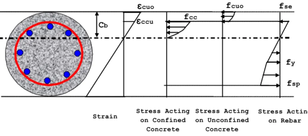
Thus in this study, a new method is proposed to plot interaction diagrams considering the confining effect by the transverse reinforcements and material nonlinearities of concrete and steel. In this method, stress in each layer of the concrete is computed from the developed concrete models in previous chapter with considering the increased strength of the confined concrete. The calculation process is illustrated in Fig. 2 for one particular strain distribution.
The maximum compressive strain ( εcou) on the outer surface of the column depends on the maximum compressive strain ( εccu) of the confined concrete and it is computed from the developed concrete model. This maximum compressive of the confined concrete is located at the contacting surface of the concrete and the transverse reinforcement.
Because the core concrete is confined and the cover concrete is unconfined, the ultimate strain of the cover concrete is much smaller than that of the core concrete. Hence, although the maximum compressive strain of the core concrete does not reach its
ultimate strain, the strain of the cover concrete may reach the ultimate strain of the unconfined concrete. At this condition, no axial force acts on the cover concrete and it is considered that the cover concrete is spalled out.
Fig. 2 Calculation of Axial Force and Moment by Proposed Method
Strain
ε ε ε εccu
Cb
fcc
fcuo
fy
fsp
fse
Stress Acting on Confined
Concrete
Stress Acting on Unconfined
Concrete
Stress Acting on Rebar
ε ε ε εcuo
The stress in the concrete is computed corresponding strain from the developed concrete models. And the forces in the concrete are computed by integrating the stresses in each layer.
And also the moments in the concrete are computed by the integrating the product of the force and the distance from the centroid at each layer. The force and moment in steel are calculated by the same process. The material model of the reinforcement is assumed a bilinear model. If the stress corresponding the strain at a certain point is larger than yield stress, it is computed considering the strain hardening of steel. If strain of steel exceeds its ultimate strain, corresponding stress in steel is zero and the corresponding longitudinal reinforcement is assumed to be ruptured. The total axial force and moment are calculated by summing the individual forces and moments in concrete and steel.
3. Derivation of Computation Method 3. Derivation of Computation Method 3. Derivation of Computation Method 3. Derivation of Computation Method
3.1 P-M Interaction Analysis Model of General Solid R.C Column 3.1 P-M Interaction Analysis Model of General Solid R.C Column 3.1 P-M Interaction Analysis Model of General Solid R.C Column 3.1 P-M Interaction Analysis Model of General Solid R.C Column
In this section the relationships is necessary to compute the various points on an interaction diagram are derived using strain compatibility and mechanics. Axil force and moment in each part of the column section are calculated and the total axial force (Pn) and total moment (Mn) are computed by summing their each component for every step which the strain distribution changes. For this calculation, bilinear models and nonlinear models are adopted as steel and concrete models respectively. And also a computer program is developed to plot interaction diagrams considering the confining effect or not.
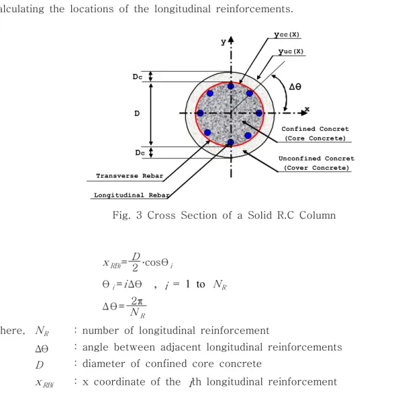
Fig. 3 shows a cross section of a solid R.C column. The diameter of the confined concrete is denoted as D and the thickness of the cover concrete is denoted as DC. If the center of the column section is set as the (0,0) point of the x-y coordinate system,
the outlines of the core concrete and the cover concrete can be defined as the functions of x. When the number of longitudinal reinforcement is NR , the angle between two adjacent longitudinal reinforcements about the center of the column will be 2π/NR. If we set the x-coordinate of the ith longitudinal reinforcement as xRBi , it is given as Eq. 1.
The diameters of the longitudinal and transverse reinforcements are neglected when calculating the locations of the longitudinal reinforcements.
Fig. 3 Cross Section of a Solid R.C Column
Transverse Rebar
x y
Dc
Dc
D
ΔθΔθΔθ Δθ yuc(X)
ycc(X)
Confined Concret (Core Concrete)
Unconfined Concret (Cover Concrete)
Longitudinal Rebar
xRBi= D
2 ․cosθi (Eq.1)
θi=iΔθ , i = 1 to NR (Eq.2)
Δθ = 2π
NR (Eq.3)
where, NR : number of longitudinal reinforcement
Δθ : angle between adjacent longitudinal reinforcements D : diameter of confined core concrete
xRBi : x coordinate of the ith longitudinal reinforcement
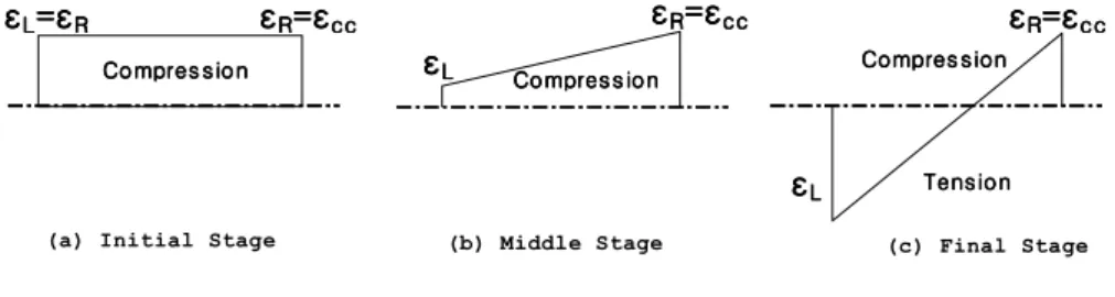
The strain of a column will be changed as the eccentricity of the load is changed. The strain of the right end of the core concrete is set as εR and its coordinate is (D/2, 0).
And the strain of the left end of the core concrete is set as εL and its coordinate is (-D/2, 0). Initially, εL and εR is equal to the peak strain (εcc) of the concrete calculated from the developed concrete model. In this stage, only axial force exists on the column without any moment. Fig. 4(a) shows this stage. If εR is fixed as εcc and εL is changed to the tensile strain, the strain distribution will be changed as shown in Fig. 4(b) and Fig.
4(c). Finally, the column fails when a longitudinal reinforcement is ruptured by tension or concrete is crushed in compression zone. In compression zone, the concrete is crushed by the rupture of the transverse reinforcement. Thus interaction diagrams can be plotted
by calculating the axial force and the moment for every stages of strain distribution.
Fig. 4 Strain Distribution
(a) Initial Stage
ε εε εRRRR=ε=ε=ε=εcccccccc
ε εε εLLLL=ε=ε=ε=εRRRR
Compres s ion Compres s ionCompres s ion Compres s ion
ε ε ε εRRRR=ε=ε=ε=εcccccccc ε
ε ε
εLLLL Compres s ionCompres s ionCompres s ionCompres s ion
ε εε εRRRR=ε=ε=ε=εcccccccc
ε ε ε εLLLL
Compres s ion Compres s ion Compres s ion Compres s ion
Tens ion Tens ion Tens ion Tens ion (c) Final Stage (b) Middle Stage
For a certain stage of strain distribution, axial forces and moments on the longitudinal reinforcements are calculated as follows. The distance between the left end of the core concrete and the ith longitudinal reinforcement ( Δxi) is given as Eq. 4. Fig. 5 shows the location of the longitudinal reinforcement and strain distribution. By calculating the strain of a longitudinal reinforcement, we can get the axial force and the moment acting on the longitudinal reinforcement.
Fig. 5 Strain Distribution on Rebar
Longitudinal Reinforcement
D
D/2
Cj
Δ ΔΔ ΔXij
εεε εR jR jR jR j=ε=ε=ε=εcccccccc
εε εεL jL jLjL jεεεεR BijR BijR BijR Bij
Fig. 6 Strain Distribution on Concrete
Cover Concrete
D
Cj
εεε εR jR jR jR j ε
εε εL jL jL jL j ε ε ε εL UjL UjL UjL Uj
ε εε εR UjR UjR UjR Uj
DC DC
Δxij= D
2 +xRB ij (Eq.4)
The slope of the strain distribution ( Δεj) is given as Eq. 5 and the strain of the ith longitudinal reinforcement ( ΔεRBij) is given as Eq. 6 at any stage of strain distribution.
Δεj= εRj- εLj
D (Eq.5)
Δε RBi= εLj+ Δεj∙Δxij (Eq.6)
where, Δxij : distance of ith longitudinal reinforcement from the left end of the core concrete along the x-axis at jth stage of strain distribution
Δεj : slope of the strain distribution at jth stage of strain distribution εLj : strain of the left far end of the confined concrete at jth stage
of strain distribution
εRj : strain of the right far end of the confined concrete at jth stage
of strain distribution
ΔεRB ij : strain of the ith longitudinal reinforcement at jth stage of strain distribution
Thus, the axial force and the moment acting on longitudinal reinforcements at jth stage of strain distribution are given as Eq. 7 and Eq. 8. Where, fRB ij is the stress on the longitudinal reinforcement which has the strain of εRB i.
P R B j= ∑
NR
i= 1f R B ij∙A n
(Eq.7)
M R B j= ∑
N R
i= 1f R B i j∙A N∙x R B ij
(Eq.8) where, AN : cross sectional area of a longitudinal reinforcement
fRB ij : stress on a longitudinal reinforcement at jth stage of strain distribution PRBj : axial force at jth stage of strain distribution
MRB j : moment at jth stage of strain distribution
For the cover concrete, the outline and the inner line of the cover concrete can be defined with functions of x as yuc(x) and ycc(x) respectively. These functions are given as Eq. 9 and Eq. 10.
yuc(x)= ( D+22Dc )2-x2 (Eq.9)
ycc(x)= ( D2 )2-x2 (Eq.10)
where, D : diameter of confined concrete Dc : thickness of cover concrete
If the strain is distributed on the column section as shown in Fig. 6 at jth stage, the axial force and the moment are calculated as follows. Where cj is the neutral axis depth at the jth stage of strain distribution in Fig. 5 and Fig. 6. This neutral axis depth cj is given as Eq. 11 from Eq. 12.
εLj= εRj cj-D
cj (Eq.11)
cj=D εRj
εRj-εLj (Eq.12)
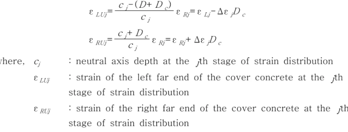
The strains of the left and right far end of the cover concrete, εLUj and εRUj , are given as Eq. 13 and Eq. 14.
εLUj= cj-(D+Dc)
cj εRj= εLj- ΔεjDc
(Eq.13)
εRUj= cj+Dc
cj εRj= εRj+ ΔεjDc
(Eq.14) where, cj : neutral axis depth at the jth stage of strain distribution
εLUj : strain of the left far end of the cover concrete at the jth stage of strain distribution
εRUj : strain of the right far end of the cover concrete at the jth stage of strain distribution
If we divide the column section into small particles as shown in Fig. 7, the area of the ith particle of the cover concrete, AUC i , is given as Eq. 15 and Eq 16. The x coordinate of the ith particle of the cover concrete is denoted as xUC i .
AUC i= 2 ⌠⌡
xUC i+ 1 xUC i
yuc(x)dx
: when x2>( D2 )2 (Eq.15) AUC i=2 ⌠⌡
xUC i+ 1
xUC i yuc(x)-ycc(x)dx
: when x2≤( D2 )2 (Eq.16) ΔxUC= D+ 2Dc
NUC (Eq.17)
xUC i=iΔxUC- D+ 2Dc
2 (Eq.18)
where, NUC : number of divided cover concrete particles ΔxUC : length of divided cover concrete particle
xUC i : x coordinate of the ith particle of cover concrete AUC i : area of the ith particle of the cover concrete
Fig. 7 Divided Section Δx
Δx Δx
ΔxUCUCUCUC ΔxΔxΔxΔxCCCCCCCC
(a) Cover Concrete (b) Core Concrete
The strain at the ith particle is given as Eq. 10 and the stress on the ith particle is the corresponding value to the given strain, computed from the developed concrete model. It is given as Eq. 19. The axial force and the moment on the cover concrete at the jth stage of the strain distribution are given as Eq. 20 and Eq. 21.
fUC(εUC i,j) =
f'co( εεUC ico,j )r
r-1 +( εεUC ico,j )r (Eq.19)
PUC j= ∑
NUC
i= 0AUC ifUC(εUC i,j)+fUC(εUC i+ 1,j)
2 (Eq.20)
MUC j= ∑
NUC
i= 0PUC ijxUC i+xUC i+ 1
2 (Eq.21)
where, εUC i,j : strain on the ith particle of the cover concrete at the jth
stage of the strain distribution
The confined concrete is divided into small particles as shown in Fig. 7(b) and the area of the ith particle of the confined concrete, ACC i , is given by Eq. 22. The x coordinate of the ith particle of the confined concrete is denoted as xCC i .
ACC i=2 ⌠⌡
xCC i+ 1
xCC i ycc(x)dx
(Eq.22) The strain at the ith particle is given as Eq. 23 and the stress on the ith particle is the corresponding value to the given strain, computed from the developed concrete mode.
The axial force and the moment on the confined concrete at the jth stage of the strain distribution are given as Eq. 26 and Eq. 5.27. The strain and the x coordinate of the longitudinal reinforcement are given by Eq. 24 and Eq. 25 in this stage.
εCC i,j= εL j+iΔεjΔxCC (Eq.23)
εCRB k,j= εL j+Δεj( D2 ․cosθk+ D2 ) (Eq.37)
xCRB k= D
2 ․cosθk (Eq.24)
PCC j= ∑
NCC
i= 0ACC i fCC(εCC i,j)+fCC( ε CC i+ 1,j)
2 - ∑
NR
k= 1AN∙fCC( εCRB k,j)
(Eq.25)
M CC j= ∑
NCC
i= 0PCC ixCC i+xCC i+ 1
2 - ∑
NR
k= 1A N∙fCC( εCRB k,j)
(Eq.27) where, εCC i,j : strain on the ith particle of the confined concrete at the
jth stage of the strain distribution
εCRB k,j :strain of the longitudinal reinforcement at the jth stage of the strain distribution
xCRB k : x coordinate of the longitudinal reinforcement at the jth stage of the strain distribution
Thus for the jth stage of the strain distribution, the total axial force and the total moment acting on the entire column section are given by Eq. 28 and Eq. 29 respectively.
The interaction diagram is obtained by plotting the point of (Mj ,Pj) at every stage of the strain distribution.
P j=PC C j+PU C j+P R B j (Eq.28)
M j=M C C j+M U C j+M RB j (Eq.29)
3.2 P-M Interaction Analysis Model of Hollow R.C Column 3.2 P-M Interaction Analysis Model of Hollow R.C Column 3.2 P-M Interaction Analysis Model of Hollow R.C Column 3.2 P-M Interaction Analysis Model of Hollow R.C Column
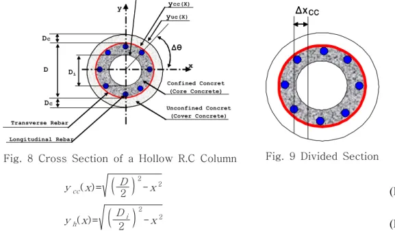
For a hollow R.C column, axial forces and moments on the cover concrete and longitudinal reinforcements are calculated by the same methods of the solid R.C column. The differences are the sectional area and the material model about the confined concrete. As shown in Fig. 8, the core concrete has a hollow section. Thus we should define the area of the confined concrete considering the hollow. The outline and the inner line of the confined concrete can be defined as the functions of x, ycc(x) and yh(x), respectively. These functions are given by Eq. 30 and Eq. 31.
Fig. 8 Cross Section of a Hollow R.C Column
Transverse Rebar
x y
Dc
Dc
D
ΔθΔθ ΔθΔθ yuc(X)
ycc(X)
Confined Concret (Core Concrete)
Unconfined Concret (Cover Concrete)
Longitudinal Rebar
Di
yh(X)
Fig. 9 Divided Section ΔxΔxΔx
ΔxCCCCCCCC
ycc(x)= ( D2 )2-x2 (Eq.30)
yh(x)= ( D2i )2-x2 (Eq.31)
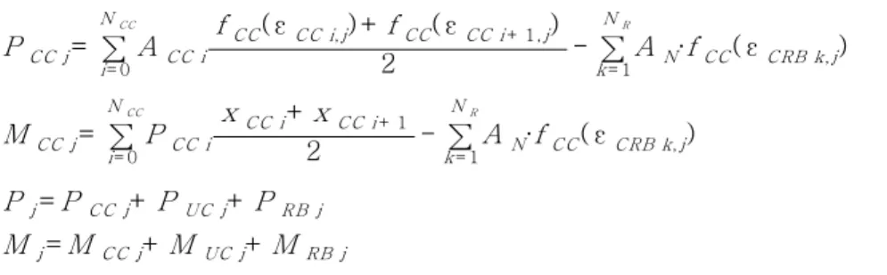
If the confined concrete is divided into small particles as shown in Fig. 9, the area of the ith particle of the confined concrete, ACC i , is given by Eq. 32 and Eq. 33. The x coordinate of the ith particle of the confined concrete is denoted as xCC i.
ACC i=2 ⌠⌡
xCC i+ 1
xCC i ycc(x)dx
: when x2>(D2i)2 (Eq.32) ACC i=2 ⌠⌡
xCC i+ 1
xCC i ycc(x) -yh(x)dx
: when x2≤(D2i)2 (Eq.33) The axial force and the moment on the confined concrete at the jth stage of the strain distribution are given as Eq. 34 and Eq. 35. Thus for the jth stage of the strain distribution, the total axial force and the total moment acting on the entire column
section are given by Eq. 36 and Eq. 37 respectively.
PCC j= ∑
NCC
i= 0ACC i fCC(εCC i,j) +fCC( εCC i+ 1,j)
2 - ∑
NR
k= 1AN∙fCC( εCRB k,j)
(Eq.34)
M CC j= ∑
NCC
i= 0PCC ixCC i+xCC i+ 1
2 - ∑
NR
k= 1A N∙fCC( εCRB k,j)
(Eq.35)
P j=PC C j+PU C j+P R B j (Eq.36)
M j=M C C j+M U C j+M R B j (Eq.37)
3.3 P-M Interaction Analysis Model of ICH R.C Columns 3.3 P-M Interaction Analysis Model of ICH R.C Columns 3.3 P-M Interaction Analysis Model of ICH R.C Columns 3.3 P-M Interaction Analysis Model of ICH R.C Columns
For an ICH R.C column, axial forces and moments on the cover concrete , confined concrete and longitudinal reinforcements are calculated by the same methods of the hollow R.C column. The difference is the material model about the confined concrete.
And we should consider the axial force and the moment on the settled internal tube.
As shown in Fig. 10, the core concrete has a hollow section and it is internally confined by the internal tube. Thus we should define strain, stress, force, moment, and geometric properties about the internal tube. The outline and the inner line of the internal tube can be defined as the functions of x, yh(x) and yt(x), respectively.
These functions are given by Eq. 38 and Eq. 39.
Fig. 10 Cross Section of an ICH R.C Column
Transverse Rebar
x y
Dc
Dc D
Δθ Δθ Δθ Δθ yuc(X)
ycc(X)
Confined Concret (Core Concrete)
Internal Tube Longitudinal Rebar
Di
yh(X) yt(X)
Unconfined Concret (Cover Concrete) t
Fig. 11 Divided Section ΔxΔx
ΔxΔxTTTT
yh(x)= ( D2i )2-x2 (Eq.38)
yt(x)= ( Di2-2t )2-x2 (Eq.39)
If the internal tube is divided into small particles as shown in Fig. 11, the area of the ith particle of the internal tube, AT i , is given by Eq. 40 and Eq. 41. The x coordinate of the ith particle of the internal tube is denoted as xT i .
AT i= 2 ⌠⌡
xT i+ 1
xT i yh(x)dx
: when x2>( Di2-2t )2 (Eq.40)
AT i= 2 ⌠⌡
xT i+ 1 xT i
yh(x) -yt(x)dx
: when x2≤( Di2-2t )2 (Eq.41) The stress on the ith particle is computed form the corresponding material model for the given strain. The axial force and the moment on the internal tube at the jth stage of the strain distribution are given as Eq. 42 and Eq. 43. Thus for the jth stage of the strain distribution, the total axial force and the total moment acting on the entire column section are given by Eq. 44 and Eq. 45 respectively.
PT j=∑
NT
i= 0AT ifT(εT i,j)+fT(εT i+ 1,j)
2 (Eq.42)
MT j=∑
NT
i= 0PT ixT i+xT i+ 1
2 (Eq.43)
P j=PC C j+PU C j+P R B j+PT j (Eq.44)
M j=M C C j+M U C j+M R B j+M T j (Eq.45)
4. Numerical Examples 4. Numerical Examples 4. Numerical Examples 4. Numerical Examples
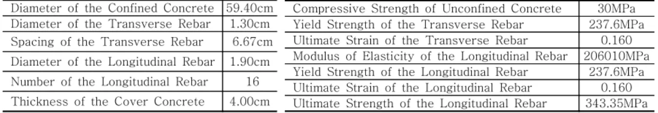
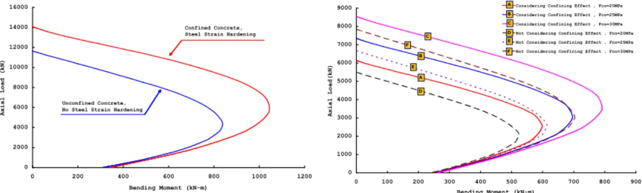
With derived equations in prior section, a computer program is coded. This program have two analysis options which consider the confining effect of the concrete and the strain hardening of the steel or not. Fig. 12 shows the difference of the interaction diagrams when the confining effect and strain hardening are considered or not. This diagrams show the current methods recommended by specifications are conservative and inaccurate because they don't consider the strength of confined concrete. The used geometric properties and material properties for analysis to plot the interaction diagrams in Fig. 12 are shown in Table 1 and Table 2 respectively.
Table 1 Section Properties
Diameter of the Confined Concrete 59.40cm Diameter of the Transverse Rebar 1.30cm Spacing of the Transverse Rebar 6.67cm Diameter of the Longitudinal Rebar 1.90cm Number of the Longitudinal Rebar 16 Thickness of the Cover Concrete 4.00cm
Table 5.2 Material Properties
Compressive Strength of Unconfined Concrete 30MPa Yield Strength of the Transverse Rebar 237.6MPa Ultimate Strain of the Transverse Rebar 0.160 Modulus of Elasticity of the Longitudinal Rebar 206010MPa Yield Strength of the Longitudinal Rebar 237.6MPa Ultimate Strain of the Longitudinal Rebar 0.160 Ultimate Strength of the Longitudinal Rebar 343.35MPa
Fig. 12 P-M Interaction Diagram of a Solid R.C Column
0 2000 4000 6000 8000 10000 12000 14000 16000
0 200 400 600 800 1000 1200
Bending Moment (kN-m)
AxialLoad(kN)
Confined Concrete, Steel Strain Hardening
Unconfined Concrete, No Steel Strain Hardening
Fig. 13 Comparison of Interaction Diagrams for Different Strengths of Concrete
0 1000 2000 3000 4000 5000 6000 7000 8000 9000
0 100 200 300 400 500 600 700 800 900
Bending Moment (kN-m)
AxialLoad(kN)
Considering Confining Effect , Fco=20MPa Considering Confining Effect , Fco=25MPa Considering Confining Effect , Fco=30MPa Not Considering Confining Effect , Fco=20MPa Not Considering Confining Effect , Fco=25MPa Not Considering Confining Effect , Fco=30MPa
A B C
D E F
A B C D E
F
Fig. 13 shows the interaction diagrams of columns which have different strengths of the concrete. The diameter of the hollow section is 40.64cm. Lines A, B, and C are the interaction diagrams considering the confining effect when the strengths of unconfined concrete are 20MPa, 25MPa, and 30MPa respectively. Lines D, E, and F are the interaction diagrams considering no confining effect when the strengths of unconfined concrete are 20MPa, 25MPa, and 30MPa respectively.
Table 5.3 Geometric Properties
Diameter of the Confined Concrete 60cm Diameter of the Transverse Rebar 1.30cm Spacing of the Transverse Rebar 5cm Diameter of the Longitudinal Rebar 1.90cm Number of the Longitudinal Rebar 12 Thickness of the Cover Concrete 4.00cm Thickness of the Internal Tube 1,2,3mm Outer Diameter of the Internal Tube 40cm Length of Corrugated Wave 6cm Height of Corrugated Wave 1.5cm
Table 5.4 Material Properties
Compressive Strength of Unconfined Concrete 20,25,30MPa Yield Strength of the Transverse Rebar 237.6MPa Ultimate Strain of the Transverse Rebar 0.160 Modulus of Elasticity of the Longitudinal Rebar 206010MPa Yield Strength of the Longitudinal Rebar 237.6MPa Ultimate Strain of the Longitudinal Rebar 0.160 Ultimate Strength of the Longitudinal Rebar 343.35MPa Yield Strength of the Internal Tube 250MPa Ultimate Strength of the Internal Tube 392.4MPa Modulus of Elasticity of the Internal Tube 206010MPa Ultimate Strain of the Internal Tube 0.160
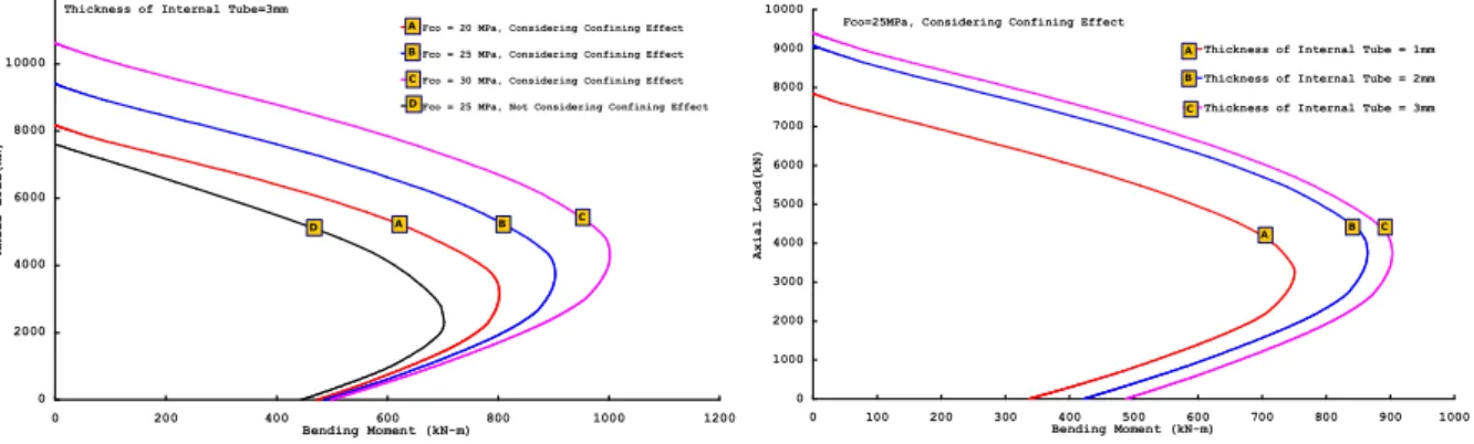
Fig. 14 shows the enlarged column strength by the increase of the concrete strength. Fig.
15 shows the enhanced column strength by the increase internal confining pressure from the internal tube. All geometric and material properties are summarized in Table. 3 and Table 4 for the columns analyzed in Fig. 14 and Fig 15.
Fig. 14 Interaction Diagrams of ICH R.C-ST Columns by the Change of Concrete Strength
0 2000 4000 6000 8000 10000 12000
0 200 400 600 800 1000 1200
Bending Moment (kN-m)
AxialLoad(kN)
Fco = 20 MPa, Considering Confining Effect Fco = 25 MPa, Considering Confining Effect Fco = 30 MPa, Considering Confining Effect Fco = 25 MPa, Not Considering Confining Effect A
B C
B C A Thickness of Internal Tube=3mm
D D
Fig. 15 Interaction Diagrams of ICH R.C-ST Columns by the Thickness of Internal Tube
0 1000 2000 3000 4000 5000 6000 7000 8000 9000 10000
0 100 200 300 400 500 600 700 800 900 1000
Bending Moment (kN-m)
AxialLoad(kN)
Thickness of Internal Tube = 1mm Thickness of Internal Tube = 2mm Thickness of Internal Tube = 3mm A
B
C
C B A Fco=25MPa, Considering Confining Effect
4. Conclusion 4. Conclusion 4. Conclusion 4. Conclusion
A nonlinear ICH R.C column model was developed considering the confining effect on the concrete of a column in this study. From the results, current specifications are too conservative and not accurate to design a reasonable ICH R.C column. Thus it is necessary to introduce the concept of confining effect on concrete for reasonable and economic ICH R.C columns. The developed nonlinear column model in this study can help to design and analyze a reasonable and economic ICH R.C column.
감사의 글 감사의 글감사의 글 감사의 글
본 연구는 한국건설기술평가원에서 시행한 『2005년도 건설핵심기술연구개발사업 과제번호( :
의 연구비 지원과 삼성물산 주 건설부문 의 부분 지원에 의하여 수행되었으며 지원
D02-01)』 『 ( ) 』 ,
기관에 깊은 감사를 표합니다.
참고문헌참고문헌참고문헌 참고문헌
1) AASHTO LRFD (1998) Bridge Design Specifications.
2) ACI Committee 318 (1999) Building Code Requirements for Structural Concrete (318-99) and Commentary (318R-99), American Concrete Institute
3) Amir Fam, Frank S. Qie, Sami Rizkalla (2004) Concrete-Filled Steel Tubes Subjected to Axial Compression and Lateral Cyclic Loads, Journal of Structural Engineering, ASCE, Apr., pp.631-640
4) J. B. Mander, M. J. N. Priestly, and R. Park (1984) Seismic Design of Bridge Piers, Research Report No. 84-2, Univ. of Canterbury, New Zealand
5) M. J. N. Priestley and R. Park (1987) Strength and Ductility of Concrete Bridge Columns under Seismic Loading, ACI Structural Journal, Title no. 84-s8, 61-76
6) T. H. Han, K. H. Han, S. Y. Han, S. N. Kim, J. O. Kang, Y. J. Kang (2005) The Behavior of an Internally Confined Hollow Concrete Filled Steel Tube Column, Proceeding of the 8th Korea-Japan Joint Seminar
7) Y. J. Kang and T. H. Han (2005) Behavior of an Internally Confined Hollow R.C Pier, Proceeding of the 8th Korea-China-Japan Symposium on Structural Steel Construction, pp.91-97