652 https://doi.org/10.9713/kcer.2019.57.5.652
PISSN 0304-128X, EISSN 2233-9558
Analytical Solutions of Unsteady Reaction-Diffusion Equation with Time-Dependent Boundary Conditions for Porous Particles
Young-Sang Cho
†Department of Chemical Engineering and Biotechnology, Korea Polytechnic University, 237, Sangidaehak-ro, Siheung-si, Gyeonggi-do, 15073, Korea
(Received 12 November 2018; Received in revised form 4 June 2019; accepted 14 June 2019)
Abstract − Analytical solutions of the reactant concentration inside porous spherical catalytic particles were obtained from unsteady reaction-diffusion equation by applying eigenfunction expansion method. Various surface concentrations as exponentially decaying or oscillating function were considered as boundary conditions to solve the unsteady partial differential equation as a function of radial distance and time. Dirac delta function was also used for the instantaneous injection of the reactant as the surface boundary condition to calculate average reactant concentration inside the particles as a function of time by Laplace transform. Besides spherical morphology, other geometries of particles, such as cylinder or slab, were considered to obtain the solution of the reaction-diffusion equation, and the results were compared with the solution in spherical coordinate. The concentration inside the particles based on calculation was compared with the bulk concentration of the reactant molecules measured by photocatalytic decomposition as a function of time.
Key words: Porous particles, Reaction diffusion equation, Eigenfunction expansion, Laplace transform, Time-dependent boundary conditions
1. Introduction
Porous particles have attracted considerable attention for their wide range of application areas, such as catalytic supports, adsorbents, membranes, and the electrode materials for energy devices [1-4].
Among them, catalytic particles have been considered as significant materials in traditional reaction engineering [5]. Currently, the porous catalytic particles are employed as various ways such as slurry-type batch reactor, packed bed reactor, or coated film-type materials for various chemical reactions in industries [6-8]. The porous nature of the catalytic particles enhances the reaction rates due to their extremely large surface to volume ratio, indicating that facile synthesis of such porous materials has been studied intensively [9]. However, the modeling and analysis of such porous particles during various chemical reactions are also important for efficient operation of reaction equipments.
For modeling and operation of catalytic chemical reactors, the monitoring of the bulk concentration of the reactant is important and such measurements are usually conducted by experimental tests. On the contrary, the concentration of the reactant inside the porous particles cannot be performed by measurements and it is essential to use modeling tool for the prediction of the behavior of the reactants inside the catalytic particles.
Thus far, several researches have been conducted to solve the reaction-diffusion equation by numerical or approximation method
[10,11]. Among them, approximate solution has been also obtained for arbitrary surface boundary condition, which requires inversion of the results from Laplace transform [12]. Analytic solution was also obtained by eigenfunction expansion method for the chemical reaction with generating chemical species, which is useful for drug delivery using biodegradable polymer [13]. However, there is a clear limitation in these previous researches, since the boundary condition at the particle surface is mainly limited to unit step function, whereas exponential decay or periodic oscillation of reactant molecules as well as instantaneous input of such chemical species can be also encountered in industrial slurry-type chemical reactors.
Thus far, the synthesis of porous particles has been carried out by various routes depending on the pore size of the particles. For instance, mesoporous particles have been fabricated by templating method by aerosol-assisted or solution phase synthesis approach [14,15].
Template-free synthesis of aerogels has been also studied by supercritical drying or under ambient pressure [16,17]. In addition to mesoporous particles, macroporous particles could be also synthesized by emulsion-assisted self-assembly approach, which was adopted in this study for the application of photocatalytic decomposition of organic contaminants [18,19].
In the present article, the concentration of reactant molecule inside the porous spherical catalytic particles was calculated by solving the reaction diffusion equation subject to time-dependent boundary conditions. The partial differential equation has been solved assuming various boundary conditions at the particle surface such as exponentially decaying or periodically oscillating function by eigenfunction expansion method. Laplace transform has been also used to solve the reaction diffusion equation for instantaneous injection of the reactant as Dirac
†
To whom correspondence should be addressed.
E-mail: [email protected]/[email protected]
This is an Open-Access article distributed under the terms of the Creative Com- mons Attribution Non-Commercial License (http://creativecommons.org/licenses/by- nc/3.0) which permits unrestricted non-commercial use, distribution, and reproduc- tion in any medium, provided the original work is properly cited.
Delta function. The effects of Thiele modulus, reaction time, and the position inside the particles have been studied to predict the concentration of the reactant inside the catalytic particles. In addition to spherical particles, the cylindrical or slab-type particles have been also considered the effect of the particle geometry. Finally, the average concentration inside the particles estimated using analytical solution has been compared with the bulk concentration of dye molecules during photocatalytic decomposition reaction using macroporous titania particles.
2. Materials and Methods
2-1. Synthesis of macroporous titania particles by colloidal templating method
The mixture of polystyrene (PS) nanospheres suspended in ethanol, titanium diisopropoxide bisacetylacetonate (TDIP), aqueous HCl solution (0.01 N) was prepared and emulsified in tetradecane containing 3 wt.% of Abil EM 90 as continuous phase. For this purpose, mechanical homogenization was carried out for 1 minute using homogenizer (hg-15a-set-a, witeg Labortechnik GmbH).
The self-assembly was induced by heating the complex fluid system at 90 °C for 1.5 hours. The produced composite particles were washed using hexane several times to remove oil phase and dried at room temperature at least for one day, followed by calcination using box furnace (Hantech, M13P) at 500 °C for 5 hours for the fabrication of the macroporous titania particles. The detailed method is described in elsewhere [6].
2-2. Synthesis of macroporous titania fibers by colloidal templating method
The PS nanospheres were redispersed in ethanol and mixed with aqueous HCl solution (0.1 N) and TDIP to prepare spinning solution.
The electrospinning was conducted by feeding the solution using syringe pump through metallic nozzle, which was connected to a power supply. The spinneret was collected onto metallic wall, and finally calcination was carried out to remove the PS nanospheres for the fabrication of macroporous titania fibers. The detailed conditions can be found elsewhere [20].
2-3. Photocatalytic decomposition of methylene blue Macroporous titania particles were suspended in aqueous medium as the concentration of 0.0002 g/ml, and mixed with aqueous methylene blue solution with 0.00002 g/ml. While the mixture was stirring, dark condition was maintained for 30 minutes for equilibration. Then, UV light was irradiated for 60 minutes and the concentration of the dye was measured with regular time intervals using UV-visible spectrometer.
The detailed method is described in elsewhere [21].
2-4. Characterizations
The morphologies of the macroporous titania particles and fibers were observed using transmission electron microscope and field
emission scanning electron microscope (FE-SEM, Hitachi-S4700), respectively. The change of bulk concentration of methylene blue was estimated using UV-visible spectrophotometer (Optizen POP) during photocatalytic decomposition of methylene blue during UV illumination.
3. Results and Discussion
Mathematical modeling to predict the reactant concentration inside porous catalytic particles was studied for three types of particle shapes such as spherical, cylindrical, and slab-type catalytic particles described schematically in Fig. 1(a), 1(b) and 1(c), respectively. Using the catalytic particles, batch-type reactor was assumed for catalytic removal of reactant molecules with three-types of boundary conditions such as exponentially decaying reactant concentration, sinusoidal and delta input of the reactant, as depicted schematically in Fig. 1(d).
In this study, the partial differential equation with time-dependent boundary condition was solved to obtain analytical solution of the reactant concentration, C(r, t). The spherical coordinate was adopted for the interpretation of the porous catalyst particles with spherical morphology. By nondimensionalization, the following reaction diffusion equation can be obtained, as explained in Supporting Information:
(1) Here, φ is the Thiele modulus, which can be defined as R(k/D
e)
0.5. By assuming initially empty catalysts, the following homogeneous initial condition can be imposed. During start-up of the catalytic reactor, this condition can be frequently found when fresh cata- lytic particles are used:
Initial Condition: y(x,0) = 0 (2)
Since the dimensionless concentration, y should be a finite value at x = 0, the following boundary condition can be written at the center of the catalyst particles. At the center of the particles, the concentration of chemical species cannot be an infinite value, thereby yielding the following zero gradient boundary condition:
Boundary condition #1: at x = 0 (3)
In this study, the boundary condition at the particle surface ( r = R or x = 1) was considered as a time-dependent boundary condition.
Three types of the boundary conditions, such as (1) exponentially decaying surface concentration, (2) periodic boundary condition, and (3) pulse-type boundary condition, were studied to solve the governing equation and obtain analytic solution. Detailed results are discussed in the following sections.
3-1. Exponentially decaying boundary condition at particle surface
As the first example, the following exponentially decaying boundary
2 2
2
1
y x y y
t x x x ϕ
∂ ∂ = ∂ ∂ ⎛ ⎜ ⎝ ∂ ∂ ⎞ ⎟ ⎠ −
0
∂ =
∂
x
y
condition was considered as the surface concentration of the reactant.
This condition can be expected during the photocatalytic degradation of organic pollutants by spherical porous photocatalytic particles under light irradiation, since the concentration of the contaminants can be reduced exponentially as a function of the UV irradiation time [21]:
(4) Here, the constant a can be determined by monitoring the change of bulk concentration of the reactant in the catalytic reaction, since 1/a can be directly related the time constant. For large value of a, the adsorbed amount of chemical species on particle surface decays rapidly as a function of time due to the depletion of the chemical species in bulk phase. If a is larger than φ, the adsorption of the reactant molecules on the particle surface can be a dominant factor than reactive depletion of the reactant, causing the rapid decrease of the reactant concentration on particle surface.
To solve the reaction-diffusion equation subject to the exponentially decaying boundary condition, the solution y(x,τ) was assumed as the summation of the functions Y
*(x,τ), R
*(τ), and u(x):
y(x,τ) = Y
*(x,τ) + R
*(τ)u(x) (5)
By substituting the above expression into the reaction-diffusion equation, the following differential equation and boundary condi- tions can be obtained:
(6)
Boundary Conditions: , (at x = 0) (7)
and (at x = 1) (8)
Initial Conditions: (at τ = 0) (9)
Now, we can set the steady-state concentration u(x) satisfies the following ordinary differential equation and boundary conditions:
(10)
Boundary Conditions: (at x = 0) and u(1) = 1 (at x = 1) (11) u(x) can be solved by assuming u(x)=U(x)/x to generate the following more simple ordinary differential equation:
(12)
It has been reported that is the steady-state con- centration of the reactant inside the porous spherical catalyst [22].
To solve Y
*, the following partial differential equation should be used for analytic solution and R(τ) should be determined:
) exp(
) , 1
( τ a τ
y = −
* * *
2 * 2
2 2
2 * 2 *
1 1
y Y dR Y d du
u x R x
d x x x x dx dx
Y R u
τ τ τ
ϕ ϕ
⎛ ⎞
∂ = ∂ + = ∂ ⎜ ∂ ⎟ + ⎛ ⎜ ⎞ ⎟
∂ ∂ ∂ ⎝ ∂ ⎠ ⎝ ⎠
− −
*
0
Y x
∂ =
∂
*
du 0 R dx =
*
(1, )
*( ) (1) exp( ) Y τ + R τ u = − a τ
*
( ,0)
*(0) ( ) 0
Y x + R u x =
2 2
2
1 d du 0
x u
x dx ⎛ ⎜ ⎝ dx ⎞ − ⎟ ⎠ ϕ = du 0 dx =
2 2
2
0
d U U
dx − ϕ =
sinh( ) ( ) sinh( ) u x x
x φ
= φ Fig. 1. (a) to (c) Schematic of porous catalytic particles with spher-
ical, cylindrical, and slab-type shapes. (d) Schematic of batch-
type catalytic reactor with particle suspension as catalyst. Reac-
tant can be injected into the slurry reactor.
(13)
In addition to the governing equation, it is necessary to find the proper initial and boundary conditions for Y(x,τ). The initial con- dition for y(x,τ) can be expressed as the following summation:
y(1,τ) = exp(-aτ) = Y
*(1,τ) + R
*(τ)u(1) (14) Assuming the homogeneous boundary condition at x = 1, Y
*(1, τ)
= 0, thus, R
*( τ) can be easily obtained due to u(1) = 1:
R
*(τ) = exp(-aτ) (15)
Thus, the partial differential equation for Y
*(x,τ) can be completely determined as the following non-homogeneous form with homo- geneous boundary conditions:
(16)
Boundary Conditions: (at x = 0) and (at x = 1) (17)
Initial Conditions: (at τ = 0)
(18) Now, Y
*(x,τ) can be obtained by eigenfunction expansion method
by defining the operator . The eigenfunc-
tion K
n(x) and eigenvalue ξ
ncan be obtained by solving the fol- lowing eigenvalue problem:
(19)
Boundary Conditions: (at x = 0) and (at x = 1) (20) Here, the eigenvalue ξ
nshould be larger than Thiele modulus ϕ to avoid the nontrivial solution Y
*(x,τ). Thus, the eigenfunction K
n(x) and eigenvalue ξ
ncan be calculated in the following way:
and ( n = 1, 2, 3, …) (21) Now, the unsteady-state solution Y
*( x, τ) can be expressed by the following eigenfunction expansion:
(22)
Here, the coefficient a
n( τ) should be obtained as a function of the dimensionless time τ to solve the reaction-diffusion equation analytically. For this purpose, the nonhomogeneous term, should be also expressed by the eigenfunction expansion method, using the following equation:
(23) Here, the time-dependent coefficient, b
n(τ), can be obtained by the following equation according to the orthogonal property of the eigenfunction, K
n( x):
(24)
Here, the inner product < K
n, K
n> can be calculated by the following way using the weight function x
2:
(25)
Similarly, can be also calculated by integration
by part to get . Thus, b
n(τ) can be obtained as the following equation for time-dependent boundary condition, aexp (-aτ):
(26)
Now, it is possible to complete the nonhomogeneous ordinary dif- ferential equation about a
n(τ) by substituting a
n(τ) and b
n(τ) as the form of the eigenfunction expansion into the partial differential equation on Y(x, τ), as the following equation:
(27)
Here, the following definition of eigenvalue problem was applied to derive the above ordinary differential equation.
(28) To obtain a
n(τ), the initial condition, a
n(0) should be known as a function of the dimensionless radial distance, x. This can be achieved from the following initial condition of Y
*(x, τ), Y
*(x,0):
(29) Due to the orthogonality of eigenfunctions, a
n(0) can be obtained by taking inner product of K
n( x) for both sides of the above equa- tion.
(30) The first order nonhomogeneous ordinary differential equation
* * *
2 2 *
2
( ) 1
Y dR Y
u x x Y
d x x x ϕ
τ τ
⎛ ⎞
∂ ∂ + = ∂ ∂ ⎜ ⎝ ∂ ∂ ⎟ ⎠ −
* *
2 2 *
2
1 exp( ) sinh( )
sinh( )
Y x Y Y a a x
x x x x
ϕ τ φ
τ ϕ
⎛ ⎞
∂ ∂ = ∂ ∂ ⎜ ⎝ ∂ ∂ ⎟ ⎠ − + −
*
0
Y x
∂ =
∂ Y
*(1, ) 0 τ =
*
( ,0)
*(0) ( ) sinh( ) sinh( )
Y x R u x x
x ϕ
= − = − ϕ
2 2
2
1 d d
L x
x dx ⎛ dx ⎞ ϕ
= ⎜ ⎝ ⎟ ⎠ −
2 2 2
2
1
nn n n
x K K K
x ∂ ∂ ⎛ x ⎜ ⎝ ∂ ∂ x ⎞ − ⎟ ⎠ ϕ = − ξ
n
0 K
x
∂ =
∂ K
n(1) 0 =
sin( )
n
( ) n x
K x x
= π ξ
n2= n
2 2π + ϕ
2*
1 1
sin( ) ( , )
n( ) ( )
n n( )
n n
Y x a K x a n x
x
τ
∞τ
∞τ π
= =
= ∑ = ∑
sinh( ) exp( )
sinh( )
a a x
x τ φ
− ϕ
1
sinh( )
exp( ) ( ) ( )
sinh( )
n n na a x b K x
x
τ φ τ
ϕ
∞
=
− = ∑
sinh( )
exp( ) , ( )
sinh( ),
( ) ,
sinh( ) , ( ) sinh( ), exp( )
,
n n
n n
n
n n
a a x K x
b x
K K
x K x
a a x
K K τ ϕ
τ ϕ
ϕ τ ϕ
< − >
= < >
< >
= −
< >
2 1 ) sin(
) ,
1sin(
0
2
=
>=
< K
nK
n∫ x x n π x x n π x dx
sinh( ) , ( ) sinh( ) x K x
nx
φ
< ϕ >
2 2 2
cos( )
n n
n
π π
π ϕ
− +
2 2 2
cos( ) )
exp(
2 )
( π φ
π τ π
τ = − − +
n n a n
a b
n2 2 2
2 2 2
( ) ( ) ( ) 2 exp( ) cos( )
n n
da n n
n a a a
d n
τ π ϕ τ τ π π
τ + + = − − π ϕ
+
2 2 2 2
( ) ( ) ( ) ( )
n n n n
LK x = − ξ K x = − n π + ϕ K x
*
1
sin( ) sinh( )
( ,0) (0)
sinh( )
n n
n x x
Y x a
x x
π ϕ
ϕ
∞
=
= ∑ = −
*
2 2 2
sinh( ) , ( )
( ,0), ( ) sinh( ) 2 cos( )
(0) ( ), ( ) ( ), ( )
n n n
n n n n
x K x
Y x K x x n n
a K x K x K x K x n
ϕ
π π
ϕ
π ϕ
< >
< >
= = − =
< > < > +
for a
n(τ) can be solved to find Y(x, τ) to obtain following analyt- ical solution y(x,τ).
(31) For a = 0, the problem can be reduced to more simple case with constant reactant concentration on the surface of the porous particles, and the initial condition of y(x,0) should be checked whether the value is equal to 0 or not, as explained in Supporting Information.
For a = 0 and ϕ = 0, the problem reduces to the simple diffusion equation without reaction, as explained in Supporting Information.
The surface concentration can be different value with the concentration of reactant in bulk fluid phase. This can be considered in the viewpoint of Biot number, which is defined as the ratio of the ratio of mass transfer resistance inside the particles and the external resistance using the following equation.
Bi = k
LR/D
e(32)
Here, k
Ldenotes the mass transfer coefficient and the mass trans- fer rate can be calculated using the following manner:
= k
L( C
b− C(R)) (33)
When Bi is small, the concentration of reactant inside the porous particles is uniform and the value is the same as the surface con- centration, since the mass transfer reissuance inside the particles is negligible. For this case, the results in this article are not nec- essary. On the contrary, the surface concentration becomes the same as the value of the reactant concentration in bulk fluid phase, as Biot number increases to large value, since the external mass transfer resistance becomes to negligible value. In this article, this situation was assumed to solve the reactant concentration inside the porous catalytic particles.
Fig. 2(a) contains the concentration distribution of the reactant inside the spherical porous particles for different values of Thiele modulus ϕ = 0.05, 0.5, 2, 5, and 50, when the dimensionless time τ and a were fixed as 0.5 and 1, respectively. In real experiment, Thiele modulus can be increased by increasing the size of the porous catalytic particles. The surface concentrations of the reactant were the same for different values of Thiele modulus, while the concentration distributions inside the particles were quite different, as shown in the graph in Fig. 2(a). For large value of Thiele modulus, the concentration of the reactant decreased as x was close to the central region of the particles, since reaction rate is much faster than the diffusion rate from the particle surface to inner region of the particles. However, the concentration of the reactant in the central region of the particles maintained relatively larger value for small value of Thiele modulus, since sufficient amount of the reactant molecule can be supplied to the inner region of the particles due to faster diffusion rate compared
to the depletion rate of the reactant by chemical reaction. Thus, the concentration of the reactant increased as the position approached to the center of the catalytic particle.
Fig. 2(b) contains the concentration distribution of the reactant inside the spherical porous particles for different values of the dimensionless time τ = 0.5, 1.5, 2.5, and 5, when the Thiele modulus ϕ and a was fixed as 5 and 1, respectively. As τ increased, the concentration of the reactant became uniform, since the concentration decreased to 0 due to the depletion of the reactant molecules.
In addition to the concentration distribution of the reactant inside the catalytic particles, the average concentration inside the particles
2 2 2
2 2 2
1
2 2 2 2 2 2
1
2 cos( ) sin( )
( , ) exp[ ( ) ]
2 cos( ) exp( ) sin( ) exp( ) sinh( )
( )( ) sinh( )
n
n
n n n x
y x n
n a x
an n a n x a x
n a n x x
π π π
τ π ϕ τ
π ϕ
π π τ π τ ϕ
π ϕ π ϕ ϕ
∞
=
∞
=
= − +
+ −
− − + −
+ − +
∑
∑
m · A ----
Fig. 2. (a) The distribution of reactant concentration y(x, τ) inside
porous spherical particles for Thiele modulus ϕ = 0.05, 0.5,
2, 5, and 50. The dimensionless time τ and a were fixed as
0.5 and 1, respectively, and the surface boundary condition
was exp(-aτ). (b) The distribution of reactant concentration
y(x, τ) inside porous spherical particles. Thiele modulus ϕ
and a were fixed 5 and 1, respectively, and the surface bound-
ary condition was exp(-aτ).
as a function of τ is also important to predict the performance of the catalyst. Thus, the volume average concentration can be calculated according to the following definition:
(34)
Since the exact solution of y(x,τ) is known for the time-dependent boundary condition as exponentially decaying function, it is possible to calculate the above integration, and the result can be obtained as the following equation:
(35)
By L’Hospital’s theorem, the first term in the above equation can be calculated when ϕ equals to 0, and the following relatively simple average concentration can be obtained for a = 1.
(36)
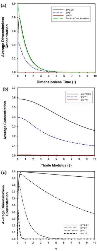
Fig. 3(a) presents the change of the average dimensionless concentration as a function of dimensionless time τ for three different values of Thiele modulus ϕ such as 0.05, 50, and 75 when a was fixed as 1. For comparison, the surface concentration was also plotted as dotted line in the same graph. When the Thiele modulus was 75, the average concentration was close to 0 regardless of τ.
However, the dimensionless concentration showed maximum value in the early stage of the catalytic reaction and decreased to 0 for lower values of the Thiele modulus such as ϕ = 0.05 and 50. Since the porous catalytic particles were assumed as initially empty state, it is natural that the average concentration increased to maximum value as τ increased, and decreased again due to the depletion of the reactant molecules by reaction and exponential decay of the reactant concentration at the particle surface.
Fig. 3(b) presents the average dimensionless concentration as a function of Thiele modulus ϕ for three different values of the dimensionless time τ = 0.5, 1, and 5. In the early stage of the catalytic reaction with small value of τ such as 0.05 and 1, the average concentration was inversely proportional to the Thiele modulus ϕ, since the reaction rate increases with increasing value of rate constant k and the Thiele modulus ϕ. However, the average concentration reduced to 0 due to the depletion of the reactant molecules at the particle surface, when τ was sufficiently large (τ = 5). The changing pattern of the dimensionless concentration was similar with the result of effectiveness factor at steady state [17].
In this study, the effect of the decreasing rate of the surface concentration y(1, τ) = exp(-aτ) was also investigated by changing the value of a and comparing the decreasing trend of the average dimensionless concentration with fixed value of ϕ = 0.05.
Fig. 3(c) presents the resulting graph as a function of the
1 2 0
( ) 3 ( , ) y τ = ∫ x y x τ dx
2
2 2 2
2 2 2 2 2 2 2 2 2
1 1
1 1
( ) 3exp( ) coth( )
exp[ ( ) ] 6 exp( )
6
n n( )( )
y a
n a a
n a n a n
τ τ ϕ
ϕ ϕ
π ϕ τ τ
π ϕ π ϕ π ϕ
∞ ∞
= =
⎛ ⎞
= − ⎜ ⎝ − ⎟ ⎠
− + −
− +
+ − + − +
∑ ∑
2 2
2 2 2 2 2 2
1 1
exp( ) 6exp( )
( ) exp( ) 6
1 ( 1)
n n
y n
n n n
π τ τ
τ τ
π π π
∞ ∞
= =
− −
= − − +
− −
∑ ∑
y τ ( )
y τ ( )
y τ ( )
Fig. 3. (a) The average dimensionless concentration as a function of dimensionless time τ for a = 1 and the surface boundary con- dition was exp(-aτ). For each graph, the Thiele modulus ϕ was fixed as 0.05, 5, and 75. (b) The average dimensionless con- centration as a function of Thiele modulus ϕ for a = 1 and the surface boundary condition was exp(-aτ). For each graph, the dimensionless time τ was fixed as 0.05, 1, and 5. (c) The average dimensionless concentration as a function of dimensionless time τ for ϕ = 0.05 and the surface boundary con- dition was exp(-aτ). For each graph, a was fixed as 0.01, 0.1, 1, and 10.
y τ ( )
y τ ( )
y τ ( )
dimensionless time τ for four different values of a = 0.01, 0.1, 1, and 10. As a decreases, the decreasing rate of the average concentration was delayed, since the surface concentration of the reactant remained relatively higher value compared to the results with larger value of a.
The dimensionless time τ
maxcorresponding to the maximum value of decreased with increasing value of a, indicating that the depletion of the reactant inside the catalytic particle could be enhanced when the surface concentration of the reactant decreased rapidly.
3-2. Periodic boundary condition at particle surface
The surface concentration of the reactant may be changed periodically, and this situation can be encountered for pressure swing adsorption. Thus, the time-dependent boundary condition with sinusoidal function was also considered to solve the reaction-diffusion equation.
For this case, the governing equation and initial/boundary conditions are the same as those of exponentially decaying surface concentration, except the following time-dependent boundary condition at x = 1:
(37) Here, the amplitude of oscillation and oscillating frequency can be determined by the constant, b and a, respectively. The reac- tion-diffusion equation can be solved by the same way, the eigen- function expansion method. Like the previous case, the steady-state concentration u(x), eigenfunction K
n(x), and eigenvalue ξ
nare the same, whereas R
*( τ) equals to 1+bsin(aτ). Thus, the partial dif- ferential for Y
*( x, τ) becomes as written in the following equation:
(38)
Here, the nonhomogeneous term can be expressed by eigenfunction expansion, as written in the following equation:
(39) Thus, the ordinary differential equation about a
n(τ), which is the coefficient of eigenfunction expansion of Y
*( x,τ), can be determined as the following nonhomogeneous equation:
(40)
To obtain a
n( τ), the initial condition a
n(0) should be determined as the following equation, in the same way as the exponentially decaying surface boundary condition.
(41) Thus, a
n(τ) can be solved as the following equation:
(42)
(43)
(44)
(45)
Now, Y
*( x,τ) can be determined to obtain y(x,τ) as the following equation:
(46) The solution, y(x,τ) with a = 0 corresponds to the dimensionless concentration with constant surface concentration, as discussed in the earlier section. For this case, the values of constants such as A, B, and C
*can be determined, and the resulting steady state solution reduces to u(x) with exponentially decaying boundary condition, as explained in Supporting Information.
y τ ( )
(1, ) 1 sin( ) y τ = + b a τ
* *
2 2 *
2
1 cos( ) sinh( )
sinh( )
Y x Y Y ab a x
x x x x
ϕ τ ϕ
τ ϕ
⎛ ⎞
∂ ∂ = ∂ ∂ ⎜ ⎝ ∂ ∂ ⎟ ⎠ − −
2 2 2
1
sinh( ) 2 cos( )
cos( ) cos( )
sinh( )
nx abn n
ab a a
x n
ϕ π π
τ τ
ϕ π ϕ
∞
=
− =
∑ +
2 2 2
2 2 2
( ) ( ) ( ) 2 cos( ) cos( )
n n
da abn n
n a a
d n
τ π ϕ τ π π τ
τ + + = π ϕ
+
*
2 2 2
( ,0), ( ) 2 cos( )
(0) ( ), ( )
n n
n n
Y x K x n n
a K x K x n
π π
π ϕ
< >
= =
< > +
* 2 2 2
( ) exp[ ( ) ] cos( ) sin( )
a
nτ = C − n π + ϕ τ + A a τ + B a τ
2 2 2 2
2 cos( )
( )
abn n
A a n
π π
π ϕ
= + +
2
2 2 2 2 2 2 2
2 cos( )
[ ( ) ]( )
a bn n
B a n n
π π
π ϕ π ϕ
= + + +
2 2 2 2 2 2 2
*
2 2 2 2 2 2 2 2
( ) ( )
2 cos( )
[ ( ) ]( )
n ab n
C n n
a n n
π ϕ π ϕ
π π
π ϕ π ϕ
+ − +
= + + +
* 2 2 2
1
( , ) [ exp[ ( ) ] cos( ) sin( )]
n
y x τ
∞C n π ϕ τ A a τ B a τ
=
= ∑ − + + +
sin( ) [1 sin( )] sinh( ) sinh( )
n x b a x
x x
π τ ϕ
+ + ϕ
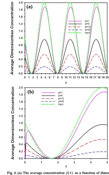
Fig. 4. (a) The average concentration as a function of dimen- sionless time τ for a = 1, b = -1, and the surface boundary condi- tion was 1 + bsin(-aτ). (b) The magnified graph of (a) in the early stage of the catalytic reaction.
y τ ( )
The average concentration inside the catalyst particles can be also derived as a function of dimensionless time or Fourier number τ by integrating y(x, τ), as written in the following equation:
(47)
Fig. 4(a) presents the change of the dimensionless concentration as a function of the dimensionless time τ for different values of Thiele modulus such as ϕ = 1, 5, 10, and 30. Here, a and b were assumed as 1 and -1, respectively, for the surface concentration y(1, τ), which was plotted as dotted line in the same graph as reference value.
As the Thiele modulus increases, the amplitude of the oscillating average dimensionless concentration decreases due to the depletion of the reactant molecules during catalytic reaction. The magnified graph in the early stage of the reaction using spherical catalytic particles is contained in Fig. 4(b). Since the catalytic particle is initially empty, the average dimensionless concentration increased from 0, causing the phase delay of the oscillating behavior. The phase delay decreased with increasing value of the Thiele modulus.
3-3. Instantaneous injection of the reactant (delta function as boundary condition at particle surface)
As the third example of the reaction-diffusion equation, the boundary condition at the particle surface can be imposed as instantaneous input as the following delta function. When huge amount of reactant is added suddenly to bulk continuous phase, the amount of the reactant molecules adsorbed on the particle surface can be considered as delta input, which can be expressed mathematically using the following Dirac delta function:
(48) This type of boundary condition can be treated by the following Laplace transform, and the exact solution can be obtained by inverse Laplace transform, rather than the eigenfunction expansion method.
(49)
The partial differential equation can be changed by Laplace trans- form, as the following manner:
(50)
Since y(x,0) equals to 0, can be obtained by solving the generalized Bessel’s differential equation. Using arbitrary constants A(s) and B(s), can be expressed as the following linear com- bination of two modified Bessel functions, I
1/2and I
-1/2.
(51)
Now, the following boundary conditions at x = 0 and x = 1 can be used to determine A(s) and B(s).
and (52)
Since I
1/2(x) = sinh(x) and I
-1/2(x) = cosh(x), the following condi- tions can be obtained.
, and B(s) = 0 (53)
Thus, the Laplace transform of dimensionless concentration y(x, τ) can be solved as the following equation:
(54)
The Laplace transform of the average concentration, can be obtained by the following integration:
(55)
By using geometric series, can be expressed as the following series, which is more convenient form to obtain the inverse Laplace transform.
(56)
Thus, can be expressed as the following equation for ϕ = 0.
(57)
The inverse Laplace transform of the above equation can be eas- ily obtained using the table from the reference book [24], and the following average concentration can be derived by applying s-shift- ing theorem.
(58)
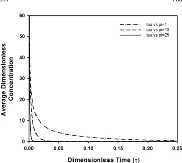
Assuming a = 1, the change of the average concentration of the reactant is plotted as a function of dimensionless time τ for three different values of the Thiele modulus ϕ, as displayed in the graph of Fig. 5. Under the instantaneous input of the reactant on the par- ticle surface, the dimensionless concentration decreases abruptly with increasing time, and the decreasing rate increases drastically with increasing Thiele modulus due to the enhancement of the reaction rate, as shown in Fig. 5.
3-4. Comparison with the results from other geometries such as cylinder or slab-type catalytic particles
In this study, the change of the average dimensionless concentration was compared for other types of the geometries of the catalytic
2
* 2 2
1
1 1
( ) 3 coth [1 sin( )]
cos( )
3 [ exp[ ( ) ] cos( ) sin( )]
n
y b a
n C n A a B a
n
τ ϕ τ
ϕ ϕ
π ϕ τ τ τ
π
∞
=
⎛ ⎞
= ⎜ ⎝ − ⎟ ⎠ +
− ∑ − + + +
y τ ( )
(1, ) ( ) y τ = a δ τ
0
ˆ( , ) ( , )exp( ) Y x s =
∞∫ y x τ − s d τ τ
2 2
2
1 ˆ
ˆ ( , ) ( ,0) d dY ˆ ( , )
sY x s y x x Y x s
x dx ⎛ dx ⎞ ϕ
− = ⎜ ⎟ −
⎝ ⎠
ˆ( , ) Y x s ˆ( , )
Y x s
2 2
1/2 1/2
( ) ( )
ˆ( , ) A s ( ) B s ( )
Y x s I x s I x s
x ϕ x
−ϕ
= + + +
ˆ(0, ) 0
Y s =
0
ˆ(1, ) ( )exp( ) Y s =
∞∫ a δ τ − s d τ τ = a
2
( )
2sinh( ) 2
A s a s
s
π ϕ
= ϕ +
+
2 2
sinh( )
ˆ( , )
sinh( )
x s
Y x s a
x s
ϕ ϕ
= +
+
( , ) y x τ
1 2
2 0 2
coth( ) 1
ˆ ( ) 3 ˆ ( , ) 3
x
Y s x Y x s dx a s
s ϕ ϕ
=
⎛ + − ⎞
⎜ ⎟
= ∫ = ⎜ ⎝ + ⎟ ⎠
coth( ϕ +
2s )
2 2
1
coth( ) 1 2 exp( 2 )
n
s n s
ϕ
∞ϕ
=
+ = + ∑ − +
Y s ˆ( )
1
1 exp( 2 )
ˆ( ) 3 2
n
Y s a n s
s s
∞
=
⎛ − ⎞
= ⎜ ⎜ ⎝ + ∑ ⎟ ⎟ ⎠
2 2
2 1
exp( )
( ) 3 1 2 exp 3 exp( )
n
y τ a ϕ τ n a ϕ τ
πτ τ
∞
=
⎛ ⎛ ⎞ ⎞
= − ⎜ + ⎜ − ⎟ ⎟ − −
⎝ ⎠
⎝ ∑ ⎠
particles such as cylindrical or slab-type pellets. Sometimes, the morphology of the catalytic particles can be chosen as cylindrical shapes as well as spherical particles [25]. The fixed bed of photocatalytic system has been also developed as slab-like films for the removal of organic dyes from aqueous medium [26]. Thus, there is sufficient motivation on the calculation from the nonspherical geometries such as cylinders and slabs.
For the case of cylindrical pellets, the time-dependent boundary condition y(1, τ) was chosen as exponentially decaying type, exp(-aτ).
The governing equations derived from cylindrical and Cartesian coordinate for cylindrical and slab-type pellets were solved by Laplace transform and eigenfunction expansion method, respectively.
The shapes of pellets were assumed as infinitely long cylinder and infinitely large slab, respectively.
In cylindrical coordinate, the solution of the following reaction- diffusion equation, y(1, τ) can be transformed to by Laplace transform.
(59)
Here, the boundary conditions are = 0 (at x = 0) and y(1,τ) = exp(-aτ), and the initial condition is y(x,0)=0. Although the eigen- function expansion approach can be applied to solve this partial differential equation, it is more beneficial to use Laplace transform method to obtain y(x, τ) from the following transformed function:
(60)
Here, Thiele modulus Φ can be defined as R(k/D
e)
0.5, when the radius of cylinder is R. The Laplace transform of the dimension- less concentration can be obtained as the following equation by applying the initial and boundary conditions.
(61)
Here, I
0denotes the modified Bessel function with zero order, which can be replaced with the Bessel function with zero order, J
0, by replacing x with ix, to apply the residue theorem. Thus, the following solution can be obtained from inversion of the above equation, for catalytic particles with cylindrical shape.
(62)
Here, λ
ndenotes the eigenvalue, which satisfies J
0( λ
n) = 0, and the values of λ
ncan be found elsewhere [27]. By integration of the above equation, the average dimensionless concentration y(τ) can be obtained as the following equation:
(63) In addition to the cylindrical coordinate, the following reaction- diffusion equation can be applied to slab-type catalytic particles subject to the same initial condition and boundary conditions.
(64) Here, Thiele modulus Φ can be defined as H(k/D
e)
0.5, when the thickness of slab is 2H. In this case, the eigenfunction expansion approach is more beneficial for solving the above equation, since the inversion after Laplace transform results in the solution y(x,τ) from integral function due to convolution theorem. Similar to the case of spherical or cylindrical pellets, zero gradient condition was imposed on the slab-type pellets at the center of the catalytic particles ( x = 0). Here, the eigenfunction K
n( x) and the steady state solution u(x) can be obtained by similar method, which was discussed in spherical catalytic particles, when the operator was
defined as .
, (65) Thus, the solution y(x,τ) and y(τ) can be obtained as the following equation:
(66) ˆ( , )
Y x s
1
2y x y y
x x x ϕ
τ
∂ = ∂ ⎛ ⎜ ∂ ⎞ ⎟ −
∂ ∂ ⎝ ∂ ⎠
y x
∂
∂
ˆ
2ˆ ( , ) ( ,0) 1 d dY ˆ ( , )
sY x s y x x Y x s
x dx ⎛ dx ⎞ ϕ
− = ⎜ ⎟ −
⎝ ⎠
0 2 0 2
( ( ) )
ˆ( , ) 1
( ( )
I s x
Y x s
s a I s
ϕ ϕ
= +
+ +
0 2 2 0
2 2
0
2 2
1 1
( ( ) )
( , ) exp( )
( ( ))
( )
2 exp[ ( ) ]
( ) ( )
n n
n n n n
I a x
y x a
I a
J x
a J
τ τ ϕ
ϕ
λ λ λ ϕ τ
λ ϕ λ
∞
=
= − −
−
− − +
+ −
∑
2 2 2
1
2 2
2 0 2 1
( ) exp[ ( ) ]
( ) 2exp( ) 4
( )
( )
n
n n
I a
y a
aI a a
ϕ λ ϕ τ
τ τ
λ ϕ
ϕ ϕ
∞
=
− − +
= − −
+ −
− − ∑
2 2
2
y y y
x ϕ
τ
∂ = ∂ −
∂ ∂
2 2
2
L d
dx ϕ
= −
( ) cos(( 0.5) ) K x
n= n − π x
2 2
cosh( ) ( ) cosh( )
u x ϕ x
= ϕ
2 2
1 2 2 2
2 2 2
2 2 2 2 2
1
cosh( ) ( , ) exp( )
cosh( )
(2 1)( 1) [ exp( ) { ( 0.5) }
exp[ { ( 0.5) } ]
[( 0.5) )][( 0.5) ]
cos[( 0.5) ]
n
n
y x a x
n a a n
n
n a n
n x
τ τ ϕ
ϕ
π τ ϕ π
ϕ π τ
π ϕ ϕ
π
−
∞
=
= −
− − − − + −
− + −
+ − + − − +
−
∑
Fig. 5. The average dimensionless concentration as a func- tion of dimensionless time for a = 1 and the surface boundary condition was aδ(τ).
y τ ( )
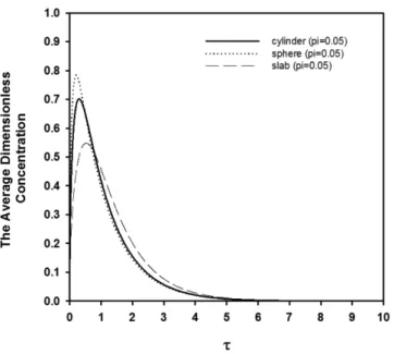
(67) Fig. 6 contains the change of the average dimensionless concentra- tion y(x,τ) as a function of dimensionless timeτ for the catalytic particles with spherical, cylindrical, and slab-type catalytic particles, for a = 1 and φ = 5. For spherical particles, the maximum value of the dimensionless concentration was the largest value among three types of morphologies, whereas the decreasing rate to steady-state value was the smallest for slab-type particles. However, the entire trend of the responses was similar regardless of the shape of the particles.
3-5. Fabrication of the catalytic particles with various mor- phologies
It has been reported that porous catalytic particles can be prepared with spherical or cylindrical morphology by colloidal templating method using polymeric beads as sacrificial templates [28,29]. Spherical catalytic particles having macropores can be fabricated by emulsion- assisted self-assembly, whereas porous cylindrical materials with very long aspect ratio can be produced by electro-spinning using polystyrene beads as templates. The fabrication process of macroporous spherical titania microparticles and macroporous titania fibers is depicted schematically in Fig. 7(a) and 7(b), respectively. The complex fluid system containing polystyrene (PS) nanospheres and titania precursor such as TDIP can be emulsified in oil phase, tetradecane which contains emulsifying agent. Since a small amount of hydrochloric acid is dissolved in the dispersed phase, hydrolysis and condensation
of TDIP can be expected during emulsion shrinkage by heating.
Then, self-organized microparticles of PS nanospheres and titania can be burnt out to form porous titania microparticles with spherical morphologies. Similarly, the suspension of PS nanospheres and TDIP can be mixed with PVP to prepare a spinning solution. During injection of the feed solution, a strong electric field can be applied for elongation of spinnerets, which can be collected on SUS sheet. After calcination, resulting macroporous titania fibers can be obtained as described schematically in Fig. 7(b).
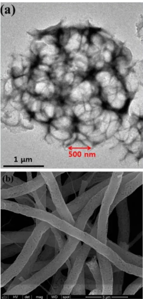
Fig. 8(a) and 8(b) contain the resulting TEM and SEM image of the spherical titania particles and electro-spun titania fibers with a number of spherical cavities, respectively. For porous titania fibers, the part of the fibrous structure can be considered as cylindrical shape with infinite longitudinal length. These porous particles can be applied to photocatalytic materials as well as catalytic supports containing metal nanoparticles for catalytic reactions [30].
The advantage of such nano-structured materials is that the tortuosity of the porous structures is relatively small, since the macropores are interconnected by tiny windows, as noted in the TEM image of Fig. 8(a). Thus, the effective diffusivity can be increased using the catalytic particles with interconnected macropores. In this sample, the spherical cavities with 1 μm in diameter are interconnected by smaller windows with about 500 nm in diameter. Thus, the mass transfer rate of reactant molecules can be enhanced through the interior region of the porous particles, which have large surface to volume ratio due to their porous nature. Large surface area can be
2 2
2 2 2 2 2 2
2 2 2 2 2
1
tanh( ) ( ) exp( )
[ exp( ) { ( 0.5) }exp[ { ( 0.5) } ]
2
n[( 0.5) )][( 0.5) ]
y a
a a n n
n a n
τ τ ϕ
ϕ
τ ϕ π ϕ π τ
π ϕ ϕ
∞
=
= − +
− − + − − + −
− + − − +
∑
Fig. 6. The average dimensionless concentration as a func- tion of dimensionless time τ for the porous catalytic particles with spherical, cylindrical, and slab-type morphologies. The parameters were fixed as a = 1 and φ = 0.05 with the surface boundary condition as exp(- aτ).
y τ ( )
Fig. 7. Schematic for the fabrication of macroporous (a) spherical
and (b) cylindrical titania particles by emulsion-assisted self-
assembly and electrospinning process, respectively.
also expected from the sample shown in the SEM image of Fig. 8(b), which presents the morphology of the macroporous titania fibers with cylindrical morphology.
In this study, macroporous titania particles with spherical morphologies were used as photocatalyst to compare the change of the concentration of methylene blue inside the particles with the concentration in bulk solution. For this purpose, porous particles having macropores with 588 nm were used as photocatalyst shown in the SEM image of Fig.
9(a). The average radius R of the porous particles was determined as 1.34 µm by measuring the size of the several particles from low magnification SEM image, as summarized in Table 1. The effective diffusivity of methylene blue in aqueous medium, D
e, was calculated as 2.2767×10
-12m
2/s by assuming the ratio of porosity and tortuosity as 0.05 and multiplying the ratio with the diffusivity D of methylene blue in aqueous medium, which was measured by microfluidic chip in other research group [31]. As the time-dependent boundary condition, the constant a was calculated as 0.00130136 using the adsorption rate constant λ, which was measured as 0.00165 sec
-1by another group according to the following Eq. [32]:
(68) Here, λ denotes the rate constant, which represents the adsorption of methylene blue on the surface of titania, assuming first-order kinetics that can be applied to various photocatalytic reactions of organic dyes as well as VOCs [32,33].
In this study, the photocatalytic degradation of the organic pollutant was monitored by measuring the concentration of organic dyes in bulk solution contained in a batch-type photocatalytic reactor. Fig.
9(b) presents the average dimensionless concentration of methylene blue as a function of UV irradiation time, which was calculated by solving a reaction-diffusion equation subject to exponentially decaying boundary condition. For this purpose, Thiele modulus Φ was calculated as 0.0204125 according to the following equation by considering the measured value of the apparent rate constant, k
app, assuming first- order reaction kinetics. Although the rate constant k inside the porous particles may be different from the value in the bulk fluid phase, k
app, it was assumed that those values are the same, indicating that the first-order rate constant is independent of the concentration of organic pollutant. Since the concentration of organic dyes used in experiment was low enough, this assumption can be reasonable for the inner and exterior region of the particles. In this article, the value of k was estimated using k
app.
(69) When the value of Thiele modulus is small, the diffusion rate is so fast that the reaction rate of reactant molecules can be considered as rate determining step, whereas the reactant is rapidly transported from bulk fluid phase to the porous particles.
The bulk concentration of methylene blue measured by experiment is also plotted in Fig. 9(b). For comparison, the average concentration of the reactant inside the particles calculated using Eq. (41) was also plotted in the same graph. Compared to the average concentration inside the porous spherical catalytic particles, the decaying rate of the bulk concentration of the dye molecules was a little bit slow, indicating that the decomposition rate of the dye molecules is relatively slower than the mass transfer rate from bulk liquid to the porous particles due to relatively slower diffusion rate than the rate of decomposition reaction. Once the reactant molecules were transported from the particle surface to interior region, the removal rate of the reactant inside the particles was predicted as a faster value, although the concentration of the reactant increased in the initial stage of the reaction, as shown in Fig. 9(b).
The limitations of the approximations in the calculations used in this study can be explained as the following points. Including the
2 e
a R D
= λ
app e