Journal of the Korean Institute of Industrial Engineers Vol. 32, No. 2, pp. 98-103, June 2006.
순서에 종속된 준비 시간과 준비 비용을 고려한 로트사이징 문제의 시뮬레이티드 어닐링 해법
정지영․박성수†
한국과학기술원 산업공학과
A Simulated Annealing Algorithm for the Capacitated Lot-sizing and Scheduling problem under Sequence-Dependent
Setup Costs and Setup Times
Jiyoung Jung․Sungsoo Park Department of Industrial Engineering, KAIST
In this research, the single machine capacitated lot-sizing and scheduling problem with sequence- dependent setup costs and setup times (CLSPSD) is considered. This problem is the extension of capacitated lot-sizing and scheduling problem (CLSP) with an additional assumption on sequence-dependent setup costs and setup times.
The objective of the problem is minimizing the sum of production costs, inventory holding costs and setup costs satisfying customers’ demands.
It is known that the CLSPSD is NP-hard. In this paper, the MIP formulation is presented. To handle the problem more efficiently, a conceptual model is suggested, and one of the well-known meta-heuristics, the simulated annealing approach is applied. To illustrate the performance of this approach, various instances are tested and the results of this algorithm are compared with those of the CLPEX. Computational results show that this approach generates optimal or nearly optimal solutions.
Keywords: lot-sizing, sequence-dependent setup costs, simulated annealing algorithm
†연락저자 : 박성수, Industrial Eng. & Management Science Bld. 373-1 Gusung-dong Yousung-gu Daejeon-si, 305-701, South Korea, E-mail : [email protected]
2005년 12월 접수; 2006년 2월 수정본 접수; 2006년 2월 게재 확정.
1.
IntroductionThe goal of this paper is to establish efficient production and inventory plan which satisfies customer’s demands with minimum overall costs including production costs, inventory holding costs and setup costs. In such competitive situations like these days, the production and inventory plan with minimum associated costs is an important issue, and modeling of the successful production plan can profit to the companies greatly. From the just-in-time (JIT) philosophy viewpoint, frequent setups are suitable for supplying the right part in right time and those can reduce inventory holding costs. However, as the number of setup grows, it can generate high
setup costs and long setup times. Hence, we have to think over production sequence and production quantity together. Despite of the intimate relations between lot-sizing and production sequence, only few attempts have been made at the capacitated lot-sizing and scheduling problem (CLSP). Moreover, most of the existing re- searches can not demonstrate the real world situations including sequence-dependent setup costs and setup times. In this paper, we consider the CLSPSD with a single machine producing multi-items over multiple periods.
The lot-sizing and scheduling problem can be classified into two different ways by the time period, i.e. macro-periods and micro period, (Drexl and Kimms). First is the discrete lot-sizing and
순서에 종속된 준비 시간과 준비 비용을 고려한 로트사이징 문제의 시뮬레이티드 어닐링 해법 99
scheduling problem (DLSP), also called the “small bucket”
problem. In the DLSP, the time periods are short and only one item can be produced per period. Second is the capacitated lot-sizing and scheduling problem (CLSP), known as the “big bucket” problem.
Multiple items can be produced during a single period in the CLSP.
In this research, we extend the lot-sizing and scheduling problem to the lot-sizing and scheduling problem with sequence-dependent setup costs and setup times. In the DLSP, Salomon et al. refor- mulated the DLSP with sequence-dependent setup costs and setup times (DLSPSD) as traveling salesman problem with time windows (TSPTW) and developed the exact solution method. On the other hand, in the CLSP, Hasse and Sungmin et al. considered the CLSP with sequence- dependent setup costs. However, they assumed that setup times are zero. Another extensive works allowing product- dependent setup times excepting for the sequence-dependent setup costs are researched by Aras et al., Trigeiro et al. and Diaby et al.
The CLSPSD is handled by Gupta and Magnusson, who provide the formulation and heuristic algorithm. However, the average deviation of the heuristic solutions from optimal solutions is too large. Therefore, we developed another simulated annealing algorithm which can be of good performance. The CLSP with setup times is the special case of the CLSPSD and it is known that the CLSP is NP-hard (Garey and Johnson). Therefore, the CLSPSD is also NP-hard. Many authors have developed heuristics to solve the CLSP and only a few attempts have been made to solve the CLSP optimally. Barany et al. reformulated the CLSP without setup times adding a strong valid inequality, and they optimally solved this problem using a Cutting Plane Algorithm. Eppen and Martin also optimally solved the multi-item capacitated lot-sizing problems using variable redefinition. Another various heuristic approaches were proposed by Mohan Gopalakrishnan et al., Kuik and Salomon and Ou Tang. In this paper, we reformulate the CLSPSD under the condition in which empty setup is not allowed, and develop the simulated annealing algorithm.
This paper is organized as follows. Section 2 describes the problem and mathematical formulation of the CLSPSD. The simulated annealing algorithm is explained in detail in section 3. In section 4, numerical examples are provided and we discuss their computational results. Finally, concluding remarks are drawn.
2. Problem description and formulation
In this paper, the capacitated single-machine multi-item lot-sizing and scheduling problem is considered. Demand,dit, for item
i = 1, ..., N over a time horizon t = 1, ..., T is given. These are dynamic and deterministic. All items must be produced on a
single machine which has finite capacity. Machine capacity is expressed in units of time. More than one item is produced in a period and if different items are produced in a single machine, setup must take place. Setup times depend on the production sequence, so-called sequence-dependent setup times, and satisfy the triangular inequality, i.e. stik+stkj≥stij for all
i, j, k = 1, ..., N, where N is the number of different items to be considered. Total costs include production costs, inventory holding costs, and setup costs. We assume that the production costs are uniform regardless of items. Setup costs also depend on the production-sequence. The object of this problem is to find feasible production plan with minimum (or close to the minimum) total costs. We suppose that the setup always starts at the beginning of the period. In other words, we do not allow the empty setup.
Furthermore, setup is kept on over idle time, i.e. setup state is not lost after idle time. We assume that machine is initially setup for some item and shortages and back-logging are not allowed. The following notation and decision variables are used to present formulation.
[Notation]
N the number of different items T the number of periods M big number
Ct the capacity of machine available in period t. Machine capacity is limited on time consumption.
dit the demand for item i at the period t
hi holding cost which is incurred to hold one unit of item i at the end of period
scij the setup cost when production change from item i to j
stij the setup time when production change from item i to j
pi the time which is needed to produce one unit of item I
[Decision variables]
qit the quantity of item i to be produced in period t
Iit the inventory of item i at the end of period t
( Ii 0= IiT= 0)
zit the machine state in period t : zit= 1, if the machine is used to produce item i in period t
xijt the setup state in period t : xijt= 1 if the machine is setup from product i to j in period t. 0, otherwise
yijt the setup state between period t and period t+1 : yijt= 1 if the machine is setup from product i to j at the beginning of period t+1. 0, otherwise
100 Jiyoung Jung․Sungsoo Park
[CLSPSD]
min ∑
N
i ∑
T
t hiIit+∑
N
i ∑
N
j ∑
T
t scij(xijt+ yijt) (1) s.t
qit+ Iit - 1= dit+ Iit ∀i, t (2)
∑
N
i p iqit+∑
N
i ∑
N
j stij(xijt+ yijt - 1)≤Ct ∀t (3)
qit≤Mzit ∀i, t (4)
xijt≤zit ∀i, j, t( i≠j) (5)
yijt≤zit ∀i, j, t (6)
xjit≤zit ∀i, j, t( i≠j) (7)
yjit≤zit ∀i, j, t (8)
i, j∈S∑ xijt≤ | S | - 1 S⊂N, 2 ≤ | S | ≤N - 1,∀t (9)
xijt+ xjit≤1 ∀i, j, t ( i ≠j) (10)
zit≤∑
j xijt+∑
j yijt≤1 ∀i, j, t ( i ≠j) (11)
zit≤∑
j xjit+∑
j yjit - 1≤1 ∀i, j, t( i≠j) (12)
∑i ∑
j yijt= 1 ∀t ( t ≠T ) (13)
xijt,yijt,zit∈ { 0, 1} ∀i, j, t (14)
qit, Iit≥0 ∀i, t (15)
The objective function (1) minimizes the sum of inventory holding costs and sequence-dependent setup costs. Constraints (2) are the inventory balancing constraints. Constraints (3) are the capacity constraints. We already mentioned that the machine capacity is defined as available operational time. Thus, finite machine capacity is further reduced by sequence-dependent setup times. Constraints (4) guarantee that production takes place only if the machine is setup for an item. Constraints (5), (6), (10) and (11) specify that exactly one setup among any setups from each of N items, j=1,…,N, to fixed item i, takes place in period t when item j is produced. Similarly, constraints (7), (8), (10) and (12) represent that just one setup among any setups from fixed item i to each of N items, j=1,…,N, occurs only if item i is produced in period t.
Constraints (9) are subtour elimination constraints: they prevent the subtours can be generated during finding a production-sequence.
Constraints (13) make sure that at least one item has to be produced per period. Finally, constraints (14) and (15) impose the binary and continuous conditions on the variables, respectively.
3. The simulated annealing algorithm
The simulated annealing algorithm was introduced by Kirkpatrick in order to solve combinatorial optimization problems. Simulated
annealing technique uses an analogous cooling operation for transforming a poor, unordered solution into an ordered, desirable solution, so as to optimize the objective function. The basic idea is to choose a neighbor randomly, and then the neighbor replaces the incumbents with probability 1 if it has a better objective value, and with some probability strictly between 0 and 1 if it has a worse objective value. Therefore, it is possible to escape from the traps of local optima. The following elements are considered in the simulated annealing algorithm :
(1) A description of possible problem solutions, so-called configuration.
(2) An objective function to measure how good any given placement configuration is.
(3) A set of random changes that will permit us to reach all feasible configurations.
(4) Cooling schedule to anneal the problem from a random solution to a good, frozen, placement.
3.1 Generation of an initial solution
To generate an initial solution, first, we decide the production lot, and determine the production sequence afterward.
(1) Determination of an initial production lot : We fix the sequence-dependent setup times to the average setup times of all setup times,st0, and ignore the sequence dependency.
We settle the production quantity of item i in period t, qit, to the demand of the item i in period t. After that, compute the total capacity used in period t. If there are any periods which violate the machine capacity, we modify the current production lot. Starting from the last period, excess capacity, so called overtime, is moved to the preceding period having available capacity. We first move the item having the lowest unit inventory holding costs and only shift the amount of production lots that are needed to get rid of overtime. We repeat this procedure until overtime has been eliminated overall periods.
(2) Scheduling the production sequence : We consider a scheduling of the production sequence in each period as the TSP and determine production sequence by applying a nearest neighbor algorithm (Cook et al.). Following is the detailed sequencing procedure. First, we generate all possible product pairs which are consist of two items representing the item which are produced in first and at last in a period respectively. Second, find the sequence which has minimum setup costs. Starting at first item, choose the next item which has the minimum setup costs while changing over from a previous item. Repeat this process
A Simulated Annealing Algorithm for the Capacitated Lot-sizing and Scheduling problem under Sequence-Dependent Setup Costs and Setup Times 101
until all items have been selected, finally reach the last item.
We store the cheapest cost to the last item in period t among those setup costs generated by all possible pairs. Between consecutive periods, select the lowest setup costs among possible setup costs. We also store the cheapest cost to the first item in next period. Repeat the previous processes in each period until reaching the last period. The cheapest accumulated setup cost out of the all setup costs at last items which are produced in last period is the total setup costs, and this sequence is the production sequence.
(3) Feasibility check : We use the feasible solution as an initial solution. Thus, we check the periods whether violate the capacity constraints or not. If there are no periods occurring excessive amount of the machine capacity, called overtimes, current solution is an initial solution. If not, we start from the last period, and shift excess production lot to the immediately preceding period having available capacity. An item which has the lowest unit inventory holding cost is shifted first. We only move the amount of the production lots that are needed to eliminate overtime. We repeat this procedure until overtime has been eliminated in all periods.
This is the initial solution. And compute the total costs.
3.2 Searching for a neighboring solution
Similar to the procedure of generating an initial solution, first we generate a neighboring production lot by moving production quan- tities, and then schedule the production sequence.
Generating a neighboring production lot : We use the amount of production quantities of item i which are produced in period t as a configuration for generating a neighboring production lot. Under the current production lots, we rearrange production lots and generate a neighboring production lot using following process.
Before rearranging production lots, we randomly choose period t1
and item i which is produced in period t1. After selecting moving period t1 and moving item,mi, we decide how many production lots move to which period, so-called target period. The mi can be moved to earlier or later period.
(1) When the total production quantity of mi from period 1 to period t1 is equal to the sum of demands of mi from period 1 to period t1 : Production lot is only moved to the imme- diately earlier period, t2, which has an available capacity.
(2) When the total production quantity of mi from period 1 to period t1 is larger than the sum of demands of mi from period 1 to period t1: Find the right after period having an available capacity,t1, and check whether the production
quantity from period t1+ 1 to period tl- 1 can satisfy the demand from period t1+ 1 to period tl- 1. If production lots satisfy those demands, the target period is t1. If not, target period is the right earlier period which has available capacity.
Now, we decide the production lots to be moved. Let the product quantity of mi in period t1 is qmit1, the available capacity in target period t2 is slackt, and △ is the production lots to be moved.
(1) If target period is earlier period :
△ = min { qit,slackt 2}
(2) If target period is later period :
△ = min
{
qit,slackt 2,τ = 1∑t1 qiτ-τ = 1∑t1 diτ}
After obtaining neighboring production lot, we determine the production sequence based on neighboring production quantities and check the feasibility of neighboring solution. This procedure is same as those which are used in the procedure of generating an initial solution.
3.3 Cooling schedule
We allow that the worse solution moves restrictively by intro- ducing the probability of acceptance, PA. The PA is calculated as follows. Let Q is an initial solution, Q' is a neighboring solution, C(Q) is objective value of a current solution, and C(Q') is objective value of a neighboring solution. Annealing temperature T is reduced when the neighboring solution increase the objective value.
A new temperature is a ×T with reduction factor a (0<a<1).
PA = exp [ C( Q) - C( Q')
C(Q)×T ]
We compare PA with a random number and if PA is greater than random number, we accept a worse neighboring solution.
3.4 A stop criterion
We complete the algorithm when the whole iteration is over the MAX_ITER or the number of iteration in a state of no improvement of solution value is over the fixed number, MAX_ITER a.
4. Computational results
To experiment the proposed algorithm, we ran a C-language in a PC with Pentium 4 (2.53GHz) with 512 MB RAM. We use
102 정지영․박성수
CLPEX 9.0 to compare our heuristic solution with optimal solution.
We randomly generate total 144 instances. The number of items range from 3 to 10 and the number of periods ranges from 3 to 10, and 20. We get the rest of the input data as follows :
(1) Demands of item i in period t, dit, are chosen out of the interval [20,60] with uniform distribution.
(2) A setup time from item i to j, stij( i ≠j), is randomly chosen out of the interval [2,10], and setup time within same items is zero, i.e. stii= 0. Setup times of a changeover from item i to j is same as the setup times of a changeover from product j to i, i.e. stij= stji, for all i,j. The choice of setup times is over so that all triangle inequalities are satisfied.
(3) We suppose the setup costs are proportional to setup times, i.e. stij= fsc×stij, for all i,j. The parameter fsc is 50.
(4) Inventory holding costs for each items,hi, are randomly chosen out of the interval [2,10] with uniform distribution.
(5) Machine capacity, C, is determined according to :
C = { 40×( number of items)} ÷ u
u is the capacity utilization and systematically differs from between 0.4 and 0.6.
(6) We set the quantity of a (Boltzmann’s constant) to 0.99 by the testing algorithms many times and select the best one which gives the best result.
(7) MAX_ITER is 2000 and MAX_ITER a is 500.
<Table 1> shows the results of our study. Let C* is the optimal value obtained by the CPLEX, and C is the objective value obtained by running the simulated annealing algorithm. And the GAP (%) is calculated as (C-C*)/C*×100. Optimal value represent the optimal solution which is obtained from using the CPLEX.
Solution value is the objective value which is obtained from solving the simulated annealing algorithm, and CPU time (sec) is running times which are needed to execute a simulated annealing algorithm. The computational results demonstrate that the average GAP is 1.39% when u=0.4 and 1.95% in case of u=0.6. These results verify that our algorithm performs well. Average running time is 34.88 sec. and 41.57 sec. respectively. If problem sizes grow bigger, getting an optimal solution using the CPLEX takes long time and we cannot obtain an optimal solution within certain time. In this case, the optimal value marked by'*'. On the other hand, our algorithm can obtain solutions in reasonable times and we also expect our algorithm will provide good results in the big size problems even though we cannot compare with the optimal solution. Finally, we compare the performance of the simulated annealing algorithm and the greedy heuristic, called ISI heuristic, which is suggested by Diwakar Gupta and Thorkell Magnusson.
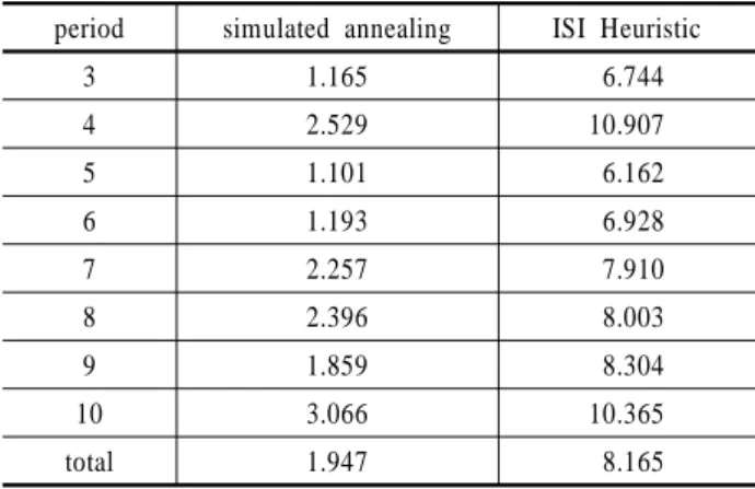
<Table 2> shows the comparison of the solutions obtained from simulated annealing algorithm and the solutions obtained from ISI heuristic. We apply the same instances which are used in simulated annealing algorithm when u is 0.6 to the ISI heuristic. Average GAP of our solution is approximately 2%, and that from ISI heuristic is approximately 8%. This result shows that our algorithm improves the solution value and provide near optimal solution.
Table 1. Summary of the computational results
u=0.4 u=0.6
period CPU time(sec) GAP(%) CPU time(sec) GAP(%)
3 18.88 1.033 20.62 1.165
4 22.03 1.147 24.52 2.529
5 18.95 1.666 29.18 1.101
6 23.71 0.930 22.73 1.193
7 34.00 1.238 39.34 2.257
8 36.29 2.208 34.71 2.396
9 38.73 0.919 40.14 1.859
10 41.97 1.997 53.41 3.066
20 79.36 * 109.51 *
Table 2. Comparison of the performance(GAP(%)) period simulated annealing ISI Heuristic
3 1.165 6.744
4 2.529 10.907
5 1.101 6.162
6 1.193 6.928
7 2.257 7.910
8 2.396 8.003
9 1.859 8.304
10 3.066 10.365
total 1.947 8.165
5. Concluding remarks
In this paper, we reformulated the CLSPSD and have introduced the simulated annealing algorithm to solve the CLSPSD. It is shown that the simulated annealing algorithm performs well and gives good feasible solution values in reasonable time. The overall average gap is approximately 2%.
Even though simulated annealing methods provide good per- formance, its computational times are slower than the running time through the CPLEX when problem sizes are small. Concerning further researches, it is still possible to improve computational time by reforming the procedure of generating neighboring solutions.
순서에 종속된 준비 시간과 준비 비용을 고려한 로트사이징 문제의 시뮬레이티드 어닐링 해법 103
Moreover, it could be of concern to research the chance of improving sequencing procedure. As based on the formulation suggested in this paper, it will be possible to obtain optimal solution or lower bound using the column generation method.
References
Aras, O. A. and Swanson, L. A. (1982), A lot sizing and sequencing algorithm for dynamic demands upon a single facility, journal of Operations Management, 2(3), 177-185.
Barany I., Van Roy, T. J., and Wolsey, L. (1984), Strong formulations for multi-item capacitated lot sizing, Management Science, 30(10), 1255-1261.
Diaby, M., Bahl, H. C., Karwan, M. H., and Ziont, S. (1992), Cap- acitated lot-sizing and scheduling by lagrangean relaxation, European Journal of Operational Research, 59, 444-458.
Diwakar Gupta, Thorkell Magnusson (2005), The Capacitated lot- sizing and scheduling problem with sequence-dependent setup costs and setup times, Computers & Operations research, 32, 727-747.
Drexl, A., Kimms, A. (1997), Lot sizing and scheduling-Survey and extensions, European Journal of Operational Research, 99, 221-235.
Eppen, G. D. and Martin, R. K. (1987), Solving multi-item capacitated lot-sizing problem using variable redefinition, Operations Research, 35, 832-848.
Garey, M. and Johnson, D. (1979), Computers and intractability : A guide to the theory of NP-completeness, Freeman and Co., San
Francisco.
Haase, K. (1996), Capacitated lot-sizing withsequence-dependent setup costs, OR Specktrum, 18, 51-59.
Kirkpatrick, S., Gelatt, Jr. C. D., and Vecchi, M. P. (1983), Optimi- zation by simulated annealing, Management Science, 220, 671-680.
Kuik, R. and Salomon, M. (1990), Multi-level lot-sizing problem : Evaluation of a simulated-annealing heuristic, European Journal of Operational Research, 45(1), 25-37.
Mohan Gopalakrishnan, Ke Ding, Jean-Marie Bourijolly, and Srimathy Mohan (2001), A Tabu-Search Heuristic for the capapcitated lot- sizing problem with set-up carryover, Management science, 47(6), 851-863.
Ou Tang (2004), Simulated annealing in lot sizing problmes, Int. J.
Production Economics, 88, 173-181.
Salomon M., Solomon M. M., Van Wassenhove L. N., Duman Y., and Duazere-Peres, S. (1997), Solving the discrete lot-sizing and sch- eduling problem with sequence-dependent setup costs and set-up times using the Travelling Salesman Problem with time windows, European Journal of Operational Research, 100(3), 494-513.
Sungmin Kang, Kavindra Malik, L. Joseph Thomas (1999), Lotsizing and scheduling on parallel machines with sequence-dependent setup costs, Management science, 45(2), 273-289.
Trigeiro W. W., Thomas, L. J., and McClain, J. O. (1989), Capacitated lot sizing with setup times, Management Science, 35(3), 353-366.
William J. Cook, William H. Cunningham, William R. Pulleyblank, Alexander Schrijver, Combinatorial Optimization.